This guest blog post was written by Max Wainwright.
In modern cosmological models, the very, very early Universe was dominated by a period of exponential growth, known as inflation. As inflation stretched and smoothed the expanding space, particles that were once right next to each other would soon find themselves at the edges of each other’s cosmological horizons, and after that they wouldn’t be able to see each other at all. It was a time of little matter and radiation — an almost complete void except for the immense vacuum energy that drove the expansion.
Luckily, at some point inflation stopped. The vacuum energy decayed into a hot dense plasma soup, which would later cool into particles and, by gravitation, conglomerate into all of the complicated cosmic structure that we see today.
The theory of eternal inflation is quite similar: the very early Universe was dominated by exponential growth, and at some point the growth needed to stop and the energy needed to be converted into matter and radiation. The difference is that in eternal inflation, the growth need not have stopped all at once. Instead, little bubbles of space could have randomly stopped inflating, or fallen onto trajectories which would lead to inflation’s end. The bubbles’ interiors would be in a lower energy state (less vacuum energy means slower inflation), and since they’re in an energetically favorable state they would expand into the inflating exterior. This is much the same as little bubbles of steam growing and expanding in a pot of boiling water: a steam bubble nucleates randomly, and then grows by converting water into more steam. If the Universe weren’t expanding, or if it were expanding slowly, each bubble would eventually run into another bubble and the entire Universe would be converted to the lower vacuum energy. But, in a rapidly expanding universe, the space between bubbles is growing even as the bubbles are themselves growing into that space. If the expansion is fast enough, the growth of inflating space will be faster than its conversion into lower-energy bubbles — inflation will never end.
Signals and Bubble Collisions
Eternal inflation is therefore a theory of many bubble universes individually nucleating and growing inside an ever-expanding background multiverse. If true, eternal inflation would mean that everything that we see, plus a huge amount that we don’t see (hidden behind our cosmological horizon), all came from a single bubble amongst an infinity of other bubbles. Eternal inflation takes the Galilean shift one step further: not only are we not the center of the Universe, but even our universe isn’t the center of the Universe! But how can we ever hope to test this theory?
Most pairs of bubble universes will never collide with each other — they’re too far apart, and the space between them is expanding too fast — but some pairs will form close enough together that they will meet. The ensuing collision will perturb the space-time inside each bubble, and, if we’re lucky, that perturbation may be visible today as a small temperature anisotropy in the cosmic microwave background (CMB).
In a recent paper with my collaborators (M. Johnson, H. Peiris, A. Aguirre, L. Lehner, and S. Liebling) we examined such a possibility. We developed a code that, for the first time, is able to simulate the collision of two bubble universes and follow their evolution all the way to the end of inflation inside each bubble. We then computed the space-time as seen by an observer inside one of the bubbles, and found what the collision would look like on his or her sky.
The model that we use starts with potential energy as a function of a single scalar field. There is a little bump at the top of the potential, forming a local minimum and a barrier. If the field is in the minimum, then it would classically stay there forever. But quantum mechanically the field can tunnel across the barrier — this is the start of a bubble universe. The field inside the bubble will then slowly roll down the potential. The interior will inflate (which is important for matching with standard cosmology), but at a slower rate than the exterior. Once the field reaches the potential’s absolute minimum and the vacuum energy goes to zero, inflation will stop and the kinetic energy in the field will convert into the hot plasma mentioned above (a process known as ‘reheating’).
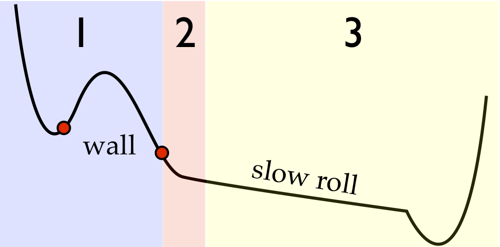
A schematic of the scalar-field potential. Region 1 controls the tunneling behavior. The field, for example, might tunnel from one red dot to another. Region 2 controls the early-time behavior inside each bubble, and therefore also controls the collision behavior between two bubbles. Region 3 controls the slow-roll inflation inside the bubble. Inflation inside the bubble needs to last long enough to solve the horizon and flatness problems in cosmology.
This next figure shows a simulation of a single collision. By symmetry, we only need to simulate one spatial dimension along with the time dimension. The x-axis is the spatial dimension, and the y-axis shows elapsed time (the time-variable N measures the number of e-folds in the eternally inflating vacuum. That is, it measures how many times the vacuum has grown by a factor of e). With our funny choice of coordinates, there is exponentially more space as we go up the graph, so even though it looks like the bubbles asymptote to a fixed size they are physically always getting bigger. You can see that collision can have a drastic effect upon the interior of the bubbles! In this case, the effect is to push the field further down the inflationary potential.
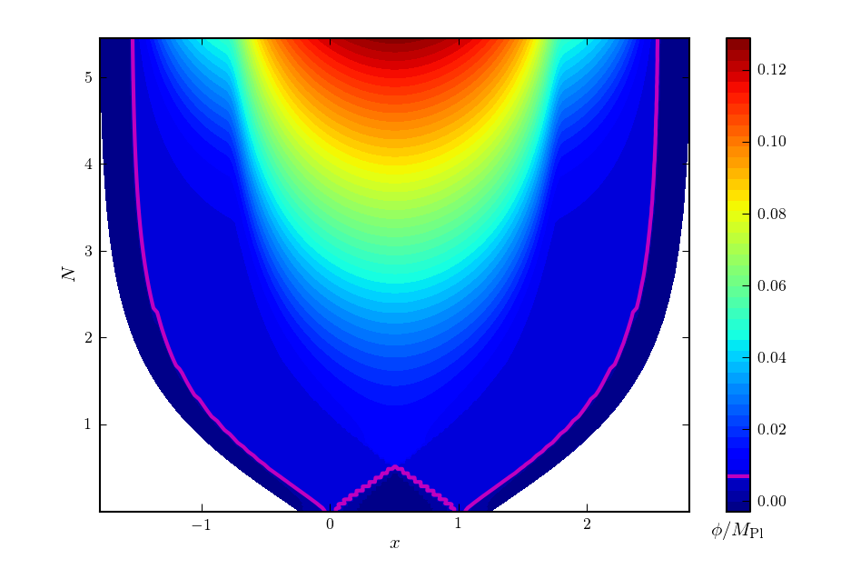
Simulation of colliding bubbles. The pink line shows the bubbles’ exteriors; white space is outside of the simulation. The different colors show different values of the scalar field.
With a collision simulation in hand, we could then figure out what collision actually looks like to an observer residing inside one of the bubbles. This step was pretty complicated — it involved a few tricky coordinate transformations and building up the observer space-time by combining many geodesic trajectories — but the end result was a measure of the comoving curvature perturbation R, which, by the Sachs-Wolfe approximation, is directly proportional to the temperature anisotropy signal that an observer would see in the CMB. The next figure shows a slice of the perturbation across an observer’s coordinates.
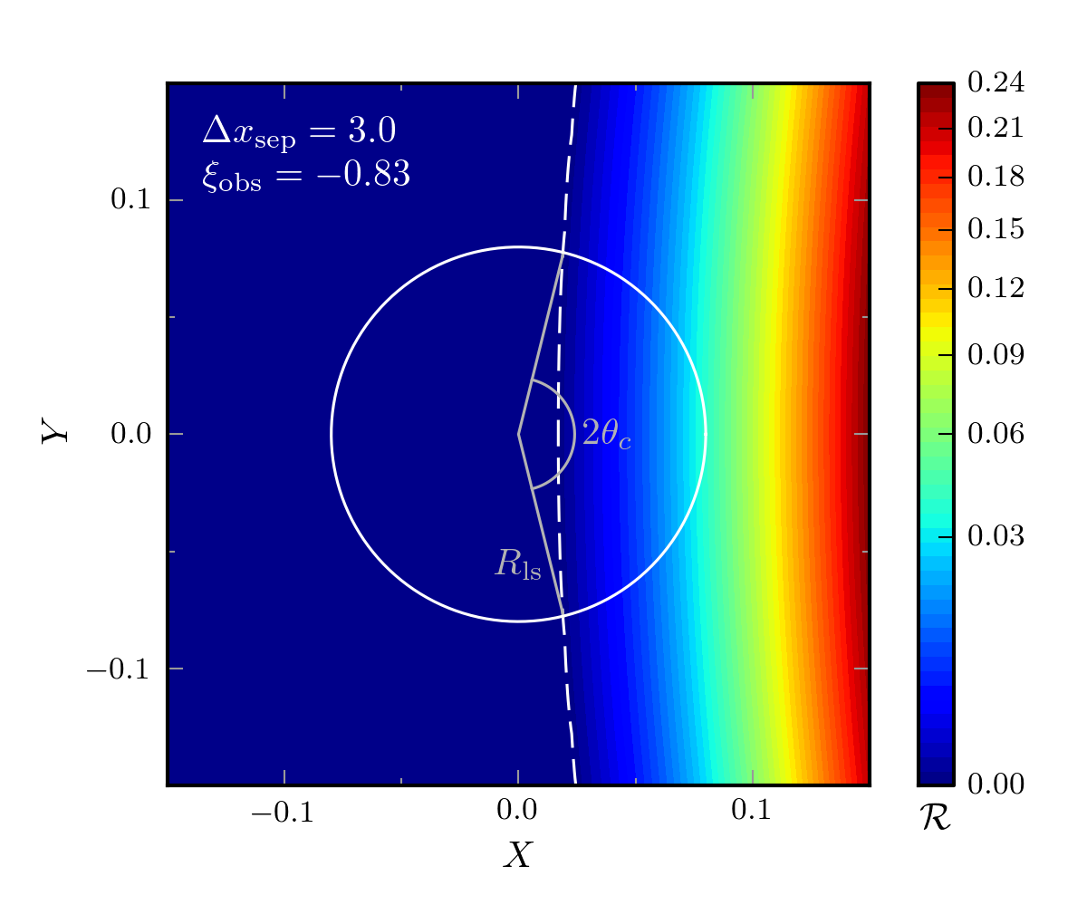
Comoving curvature perturbation near an observer. The perturbation is azimuthally symmetric (symmetric about the X-axis), so the Z-axis does not need to be shown. An observer would see the perturbation on the slice of their past light-cone which intersects the surface of last scattering (the space-time surface from which the CMB is emitted). In the two dimensions plotted here, that surface would (for example) coincide with the circle surrounding the origin. In three dimensions, the collision would look like a big slightly bright spot on one side of the CMB sky.
Predictions and Next Steps
What I’ve shown here is the result of a single bubble collision for a single observer, but, as shown in the paper, we ran many different collisions with different initial separations between bubbles, and found the resulting signal for many different observers. This allowed us to make robust predictions for what sizes and shapes of collisions we should expect to see, given this model. We will then use this information to actually hunt for the collision signals in the sky using data from the Planck space observatory.
So far we’ve only examined one model for how the scalar-field potential should look, but we have no strong theoretical bias to believe that that model is right. Now that we have all of the machinery, we can start examining a slew of different models with different collision properties. Will the collisions generically look the same, or will different models predict very different signals? If we find a signal, what models can it rule out?
It’s an exciting time to be a cosmologist. If we’re lucky, we may soon learn of our proper place in the multiverse.
You can read more here:
C. L. Wainwright, M. C. Johnson, H. V. Peiris, A. Aguirre, L. Lehner, S. L. Liebling
Simulating the universe(s): from cosmic bubble collisions to cosmological observables with numerical relativity
M. C. Johnson, H. V. Peiris, L. Lehner
Determining the outcome of cosmic bubble collisions in full General Relativity
S. M. Feeney, M. C. Johnson, J. D. McEwen, D. J. Mortlock, H. V. Peiris
Hierarchical Bayesian Detection Algorithm for Early-Universe Relics in the Cosmic Microwave Background
