This guest blog post was written by Layne Price.
The cosmological principle says that our universe looks the same regardless of where we are or in which direction we look. Obviously, a universe that exactly satisfies this principle is unimaginably boring, precisely because we wouldn’t be here to imagine it. In fact, a quick measurement using my bathroom scale and a tape measure suggests that I have a density around 1100 kg/m3, which is 1030 times larger than the cosmological average. Clearly, the universe is homogeneous and isotropic only when averaged over large-enough scales. So, where do the local differences in density come from?
Enter inflation. This is a class of theories that uses the inherent randomness of quantum perturbations to generate local fluctuations in the dominant energy component of the primordial universe: hypothesized quantum fields with no intrinsic spin. Fields of this type are called scalars and show up often in physics: phonons in solid state physics are scalars, as is the recently discovered Higgs boson. The random fluctuations in these scalar fields cause small changes in the spacetime curvature, collecting dark matter and baryons into regions of space which eventually collapse into galaxies, stars, and people.
Although the local curvature perturbations are random, not all randomness is equal. The different possible variances of the random curvature perturbations are distinguishable through the shape of the acoustic peaks in the angular power spectrum of the cosmic microwave background (CMB). For example, if the perturbations were pure Gaussian white noise, then there would be more power on smaller angular scales than has been seen by the WMAP and Planck satellites. This simple type of randomness has now been eliminated at a level greater than 5 sigma.
Interestingly, inflation predicts a small, but non-negligible deviation from white Gaussian noise, which is exactly what we see. However, the amount and type of this deviation depends on the way the scalar field theory is constructed — and there are lots of ways to make scalar field theories. If there is only one scalar field, there is usually only one way to inflate: one field using its potential energy to drive the universe’s expansion, which in turn acts as a frictional force to stop the field from gaining too much momentum. This causes a runaway effect where the expansion becomes progressively faster, sustaining inflation for an extended period of time. Since single-field models depend only on the potential energy of one field, for every potential energy function there is usually a unique prediction for the statistics of the CMB.
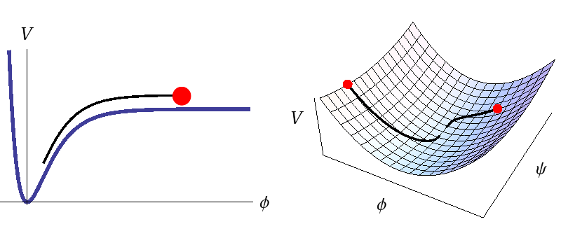
This shows the scalar field potential energy density V as a function of one field (left) or two fields (right). The red dots indicate some possible initial positions for the fields, while the black lines show the paths the fields would take during inflation. With one field you can only go one way down the potential; all initial conditions give the same outcome. With more than one field the paths are different for different initial conditions and each of these predict slightly different statistics for the CMB.
However, fundamental particle physics theories, like string theory or supersymmetry, often have hundreds or thousands of scalar fields. Since these theories become most relevant at energy scales close to the inflationary energy scale, there is considerable interest in analyzing their dynamics. This certainly complicates things. Multifield models have not only one, but usually an infinite number of ways to inflate. The potential energy that drives inflation can now be distributed across any combination of the fields and this distribution of energy changes during the inflationary period in complicated ways that depend on the fields’ initial conditions. The dynamics can even be chaotic! With so many more degrees of freedom, multifield models give a much wider range of possible universes. Understanding whether or not our universe fits into this spectrum is obviously a big challenge!
To determine the predictions of multifield models it is therefore useful to employ a numerical approach that can handle their increased complexity. Over a few visits back-and-forth between London and Auckland, my collaborators and I have built an efficient numerical engine that can solve the exact equations describing the inhomogeneous perturbations. The speed of the code has allowed us to calculate statistics for models with over 200 scalar fields — many more than previously possible. Perhaps surprisingly, our calculations indicate that the most likely predictions of the multifield models are bunched tightly around tiny regions of parameter space and are not sensitively dependent on the initial conditions of the fields.
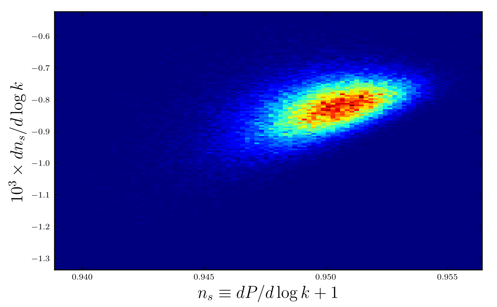
This is a 2D histogram where blue and red indicate less-likely and more-likely regions, respectively. We have used 100 fields to drive inflation and have looked at 100,000 different initial conditions. But first, some basics: simple inflation models predict density perturbations that are random and the density’s modes at a given physical scale, or wavenumber k, are drawn from a Gaussian probability distribution with a variance equal to the primordial power spectrum P(k). A perfect white noise spectrum has P=constant. So, I have plotted here the first and second derivatives of P with respect to the logarithm of k. Although the possibilities for this multifield model are widely varied, the vast majority of our results are grouped tightly together, indicating that the initial conditions are less important than one might expect.
This is important because, in order to calculate how much the observations favor a given model, we need to sample the entire relevant portion of the model’s parameter space and weight each combination of parameters according to how well they fit our CMB observations. This process is computationally difficult, so if we can argue that the fields’ initial conditions only weakly affect the model’s predictions, then it allows us to use a smaller sample, greatly simplifying the calculation.
The end-goal of this line of research is to know which animal in the zoo of inflation models, if any, gives the best description of our universe. For each of these models we must individually calculate the probability that the model is true given the data we have extracted from the CMB — in Bayesian statistics this is known as the posterior probability for the model. By taking the ratio of two models’ posterior probabilities we can determine which model we should bet on being the better description of nature. While we still have more work to do before we can calculate which multifield inflation model is best, we now have many efficient tools in place. There will be much more to come soon!
You can read more here:
R. Easther, J. Frazer, H. V. Peiris, and L. C. Price
Simple predictions from multifield inflationary models
R. Easther and L. C. Price
Initial conditions and sampling for multifield inflation
