This blog post was written by Andrew Pontzen.
Over this year, a few of us at UCL have been getting increasingly interested in the Lyman alpha forest. It’s a unique probe of how gas is distributed through the universe, made possible by analysing the light from distant, bright quasars. While a lot of emphasis has been placed on the ability of the distribution of gas to tell us about dark energy, we’ve been making the case that there’s more information lurking in the raw data — more here in UCL’s official press release and blog.
For press purposes our work has been illustrated by a picture from an ongoing computer simulation. But actually, one of the neatest aspects of this work is that it can be done with pencil and paper. We’ve built a rigorous framework to study how light propagates through the large-scale universe, without running a conventional simulation. Over the coming months and years we hope to build on that framework to study more about how the large scale universe is reshaped by the light streaming through it.
You can read more here:
UCL press release
What lit up the universe?
A. Pontzen
Scale-dependent bias in the BAO-scale intergalactic neutral hydrogen
A. Pontzen, S. Bird, H. Peiris, L. Verde
Constraints on ionising photon production from the large-scale Lyman-alpha forest
Wikipedia
The Lyman-alpha forest
The DESI Collaboration
The DESI Experiment, a whitepaper for Snowmass 2013
Neutrinos: cosmic concordance or contradiction?
Our recent paper on possible new physics in the neutrino sector from cosmological data has been selected as an Editor’s Suggestion in Physical Review Letters! The work was discussed in comprehensive blog posts at phys.org and on the UCL Science Blog; a recent guest post on the topic at Early Universe @UCL is here.
Is the universe a bubble? Let’s check!
The Perimeter Institute did a major press release on our new work in simulating bubble collisions in eternal inflation in full General Relativity. The accompanying video has garnered over 100k views on YouTube! The story was covered in phys.org and IFLScience. A guest post on this topic was previously featured on Early Universe @UCL.
This guest blog post was written by Stephen Feeney.
The cosmic microwave background (CMB) forms the cornerstone of the concordance cosmological model, ΛCDM, providing the largest and, arguably, cleanest-to-interpret picture of our Universe currently available; however, this model is buttressed on all sides with measurements of cosmologically relevant quantities derived using a huge variety of other astrophysical objects. Examples include:
-
the local expansion rate of the Universe (i.e., the constant in Hubble’s Law relating the distance of an object and its recession speed), measured using so-called standard candles — things we (think we!) know the inherent brightness of — such as Cepheid variable stars and Type Ia supernovae;
-
the age of the Universe, which must be greater than the ages of the oldest things we can see, like globular clusters and metal-poor stars; and
-
the shape or amplitude of the matter power spectrum, i.e., how much matter, (both normal and dark) is bound up in structures of different sizes. This can be measured in a number of different ways, including galaxy surveys, weak-gravitational-lensing surveys (which exploit the fact that matter bends the path of light, and hence changes the shape of faraway objects, to “weigh” the Universe) and counts of galaxy clusters.
Using our cosmological model, we can extrapolate our CMB observations — observations of the Universe when it was only 400,000 years old — to predict how quickly we think the Universe should be expanding now (billions of years later), how old it should be, and how many galaxy clusters we should see of a given mass. If our model of cosmology (and crucially astrophysics — more on this below) is correct, and we truly understand our instruments, then all of our measurements should agree with the CMB predictions. Conversely, if our measurements don’t agree then we might have something wrong! With releases of stunning new cosmological data popping up more regularly than a London bus — ain’t being a 21st century cosmologist great? — there’s no time like the present to ask just how concordant is our concordance model?
Now, the first thing to note is that our measurements very nearly do agree. Let’s take the expansion rate as an example. Extrapolating the Planck satellite’s CMB observations to the present day, we expect that the expansion rate should be 67.3 ± 1.2 km/s/Mpc (the slightly funky units reduce to 1/s, the same as any old rate). The Hubble Space Telescope’s dedicated mission to measure this quantity, which used observations of some 600 Cepheid variables and over 250 supernovae, concluded that the expansion rate is 73.8 ± 2.4 km/s/Mpc. The level of agreement between these two values is pretty mind-blowing, particularly when you consider we’re talking about modelling a few billion years of cosmological evolution. We’re comparing predictions based on observations of the Universe when it was a soup of photons, protons, electrons, a few alpha particles and not much more to measurements of pulsating and exploding stars! Put simply: it looks like we’re doing a good job!
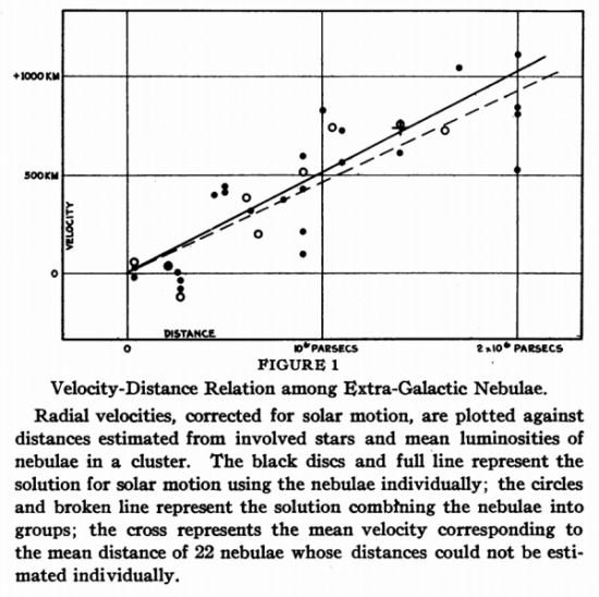
Hubble’s original measurement of the local expansion rate: we’ve come a long way since!
When we compare the difference between these two values with the errors on the measurements, however, things look a little less rosy. Even though the values are close, their error-bars are now so small that this level of disagreement indicates we don’t understand something important, either about the data or the model. Or, of course, both. Looking elsewhere, we see similar issues popping up. Though our measurements of the age of the Universe look ok compared to the CMB predictions, estimates of the amount of matter from cluster counts (and weak-lensing measurements) suggest that there isn’t as much small-scale (cosmologically speaking) structure as we’d expect from extrapolating the CMB.
So far, so mysterious. Luckily though there are (plenty of!) models waiting to explain the discrepancy. What we’re looking for here are processes that can make the current Universe deviate from the predictions of the early Universe, things like massive neutrinos, dark energy and the like, whose effects only show up once the Universe has reached a certain age. Massive neutrinos have been receiving a lot of attention recently, with several papers reporting tentative detections of the existence of an additional massive sterile neutrino species (“sterile” here meaning that the neutrinos don’t even interact via the weak nuclear force: these are some seriously snooty particles…). Where does the evidence for these claims come from? Well, the effects of sterile neutrinos on cosmology can be described by their temperature and mass, which govern when the neutrinos are cool enough to stop behaving like radiation (pushing up the expansion rate and damping small-scale power) and instead start behaving like warm dark matter. Warm dark matter, unlike its cold cousin, moves too quickly to cluster on small scales, and thus suppresses the formation of cosmological structure. If a population of sterile neutrinos was produced in the Big Bang, and it became non-relativistic after the CMB was formed, the matter power spectrum on these scales would be smaller than that predicted by the CMB.
Okay, so it looks like an extra sterile neutrino could explain the paucity of clusters in the Universe. Nobel Prizes all round! Except that’s not the whole story. A Universe with three normal neutrino species and an extra sterile one should have a low Hubble expansion rate as well as low cluster counts: that is not what is observed. Quite the opposite, in fact, as we’ve seen: a range of local measurements of the Hubble constant point to a value higher than expected. Thus, it appears that the sterile neutrino model does not provide the new concordance we all crave. This point has been very nicely illustrated in a recent paper by Boris, Hiranya and Licia, who demonstrate (using the data mentioned above and more) that adding a sterile neutrino to the standard cosmological model can not reconcile the high local measurement of the Hubble rate and the low cluster counts with the predictions of higher-redshift data from CMB observations (which by themselves don’t seem to want anything to do with massive neutrinos). In scientific terms, the datasets remain in tension, and we all know what happens when we combine data that are in tension: if there is only a small overlap between the conclusions of each dataset, we end up with artificially small ranges of allowed parameter values.
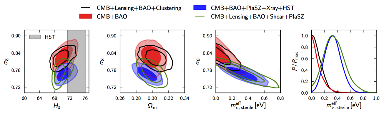
Figure from Leistedt et al. showing the tension between CMB and cluster data. The plots show the most probable values of the Hubble expansion rate, H0, the total amount of matter, Ωm, a measure of the amplitude of the matter power spectrum, σ8, and the effective mass of the sterile neutrino, mν, when different data are considered. The large shift in allowed parameter values when cluster (PlaSZ/Xray) and expansion-rate (HST) data are added to CMB data indicates that these measurements do not agree even when an additional sterile neutrino species is added to the standard cosmological model.
What else could explain the discrepancy then? Well, firstly and most excitingly, we could have the wrong model. Perhaps there is another physical process taking place on cosmological scales that perfectly predicts all of our observables. If this is the case, this is where Bayesian model selection comes into its own: once we have the predictions of this model, we can easily test whether the model or its competitors is most favoured by the data. (Of course, Bayesian model selection already has a part to play: it’s a more naturally cautious method than parameter estimation, and even using the current data in tension it shows that the sterile neutrino model isn’t favoured over ΛCDM.)
The other possibility is that there are undiagnosed systematic errors in one or more of the datasets involved. This is not an outlandish possibility (and historically this is where confirmation bias raises its ugly head): the measurements we’re discussing here are all hard to do, and are rarely free from interference from astrophysical contaminants. It’s very easy to only focus on the cosmological quantities derived from these observations, and just chuck them into your analysis as a number with some error-bars, but it’s important to remember that each of these numbers is itself the distillate of a complicated astrophysical whodunit. Like detectives using clues and logic to piece together the most likely story of what happened, we use observations and physical theory to figure out the most probable values of the cosmological parameters. The values of the parameters therefore depend on how well we understand both our data and the objects we observe. Measurements of the local expansion rate rely on standard candles: we need to understand the physical processes that determine the brightness of these objects, and how dust or metals in their surroundings might affect that brightness. To derive measurements of the matter power spectrum we need to understand how galaxies (and not only galaxies in general, but the specific ones we see in our surveys) map onto the dark matter distribution, how all of this evolves as structures collapse under gravity, how the amount of X-rays emitted by a cluster relates to its mass, how the shapes of galaxies are warped by intervening matter (and are distributed in the first place!). For age measurements we need to understand how stars evolve and impact the formation of new stars in their surroundings, etc., etc. Are we sure, for example, that our conversion from cluster counts (or the amount of X-rays radiated by clusters) into the amplitude of the matter power spectrum is exactly correct? How confident are we that the standard candles used to measure the local expansion rate are truly standard (i.e. could variations in these objects mean some are actually inherently brighter than others), or that the calibrations between different candles are correct? And what if our understanding of the instruments aboard the Planck satellite is not perfect? Tweaking any one of these could cause our measurements of the cosmological parameters to shift (and in any direction: there’s no guarantee they will move into agreement!). We need to dig around our data to determine whether any instruments are misbehaving, and test both the physical principles and statistical tools used to convert our data into constraints on cosmological parameters to be sure that this isn’t the source of the discrepancy.
So, this is where we find ourselves today. It seems recently that everyone’s re-examining everyone else’s data: the expansion rate calculations have been revisited by Planck people, and the Planck power spectrum analysis has been tweaked by WMAP people, each potentially resulting in small but important shifts in parameter values. And the good news is that no punches are being thrown (yet!). I find this to be very cool, and very exciting: we’re not all sitting here agreeing; neither are we all flatly claiming our data are error-free; nor are we blindly accepting that claims of new physics are true, as awesome as it would be if they were. The next year or so, in which these re-examinations are in turn examined and, more importantly, new temperature and polarisation data from the Planck satellite appear, will subject our cosmological models to extremely exacting scrutiny to truly determine whether concordance, be it new or old, can be found.
You can read more here:
Planck Collaboration
Planck 2013 Results. XVI. Cosmological Parameters
H. Bond, E. Nelan, D. VandenBerg, G. Schaefer and D. Harmer
HD 140283: A Star in the Solar Neighborhood that Formed Shortly After the Big Bang
A. Riess et al.
A 3% Solution: Determination of the Hubble Constant with the Hubble Space Telescope and Wide Field Camera 3
R. Battye and A. Moss
Evidence for Massive Neutrinos from CMB and Lensing Observations
C. Dvorkin, M. Wyman, D. Rudd and W. Hu
Neutrinos Help Reconcile Planck Measurements with Both Early and Local Universe
B. Leistedt, H. Peiris and L. Verde
No New Cosmological Concordance with Massive Sterile Neutrinos
S. Feeney, H. Peiris and L. Verde
Is There Evidence for Additional Neutrino Species from Cosmology?
G. Efstathiou
H0 Revisited
D. Spergel, R. Flauger and R. Hlozek
Planck Data Reconsidered
This blog post was written by Marc Manera.

This is the 2.5 meter telescope used by the SDSS collaboration at the Apache Point Observatory
More than one million galaxies have been observed in the last three years by the 2.5 meter telescope at the Apache Point Observatory in New Mexico. In the picture above you can see the telescope (and me) just before sunset during a visit I made to the observatory some years ago. Some of the astronomers and cosmologists of the Sloan Digital Sky Survey had met nearby to discuss the science that can be done with the forthcoming observations – but now the data are already here.
When you have observations of the position and colour of more than one million galaxies at your fingertips, there are a lot of questions about the universe that can be investigated. In this post I will focus on how we have measured the expansion of the universe using the distribution of galaxies from the BOSS survey, which is part of the Sloan Digital Sky Survey.
BOSS – the Baryon Oscillation Spectroscopic Survey – has targeted 1.35 million galaxies covering approximately 10,000 square degrees. Galaxies are observed by setting optical fibres in the focal plane of the telescope. The light of each galaxy is then carried to a spectrograph where it is diffracted into a spectrum of wavelengths or frequencies i.e. colours – like a rainbow – and the data are stored.
As the light travels from the galaxy where it was originally emitted to us, the spectrum of colours of the galaxies shifts towards the red; i.e., the galaxies appear “redder” than their original colour. We call this change in colour redshift, and we can measure it because we know the colour/frequency of a particular atomic transition as it would have been observed in the galaxies when it was emitted. The magnitude of the colour change – the redshift – is an important cosmological quantity, and tells us how much the universe has changed in size since that light was emitted. If the universe has doubled its volume since then, then the wavelength of the light that we observe will have doubled too.
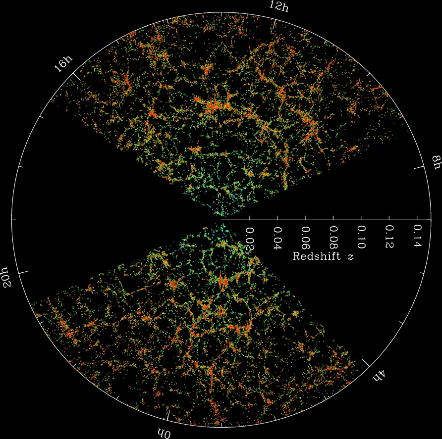
This is a map of some of the galaxies observed from the SDSS telescope. Courtesy of M Blanton and the Sloan Digital Sky Survey
The figure above shows slices through the SDSS 3-dimensional map of the distribution of galaxies. The Earth is at the centre, and each point represents a galaxy, typically containing about 100 billion stars. The outer circle is at a distance of 2 billion light years. The wedges showing no galaxies were not mapped by the SDSS because dust in our own Galaxy obscures the view of the distant universe in this direction. Both slices contain all galaxies between -1.25 and 1.25 degrees declination.
As the SDSS map shows, galaxies in the universe are not distributed randomly. Galaxies tend to cluster in groups of galaxies because they attract each other through gravity. Galaxies also have a particular separation at which they are more likely to be found; this separation is set by plasma physics – it is the Baryon Acoustic Oscillation characteristic distance – and we know it is about 4.5 x 10²¹ km. This is the distance that galaxies “like” to keep between themselves, in a typical sense.
In the sky, for each set of galaxies that emitted their light at a particular moment during the expansion of the universe, the typical separation of the galaxies subtends a particular angle. Since we can calculate this separation between galaxies from physics (r) and the angle it subtends by observation (θ), using the basic geometry of a triangle we can work out the distance between us and these galaxies (d). This is illustrated in the final figure below.
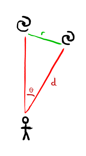
This shows a person observing two galaxies separated by a typical distance r. If we know then angle θ, we can measure the distance from us to the galaxies.
Finally, because the speed of light in constant, we know how long ago the light from the galaxies was emitted, and thus we have all the information we need to deduce the expansion history of the universe.
So to sum up, to work out the expansion rate of the universe we select several samples of galaxies; each sample will have emitted its light at a different time, and therefore it is at a different distance to us. We can measure this distance using simple geometry by observing the typical angle by which galaxies are separated. Once we have the distance to each sample of galaxies, we also have a measure of how long ago they emitted that light. Now, from the colours of the galaxies (the redshift) we also know how big the universe was at that time. For each set of galaxies we know the age of the universe at a particular moment and how big the universe was at that time. We have therefore determined the expansion history of the universe.
This is exactly what the BOSS survey has done using three sets of galaxies at different distances.
You can read more here:
L. Anderson, E. Aubourg, S. Bailey et al (BOSS collaboration paper)
The clustering of galaxies in the SDSS-III Baryon Oscillation Spectroscopic Survey: Baryon Acoustic Oscillations in the Data Release 10 and 11 galaxy samples
This guest blog post was written by Layne Price.
The cosmological principle says that our universe looks the same regardless of where we are or in which direction we look. Obviously, a universe that exactly satisfies this principle is unimaginably boring, precisely because we wouldn’t be here to imagine it. In fact, a quick measurement using my bathroom scale and a tape measure suggests that I have a density around 1100 kg/m3, which is 1030 times larger than the cosmological average. Clearly, the universe is homogeneous and isotropic only when averaged over large-enough scales. So, where do the local differences in density come from?
Enter inflation. This is a class of theories that uses the inherent randomness of quantum perturbations to generate local fluctuations in the dominant energy component of the primordial universe: hypothesized quantum fields with no intrinsic spin. Fields of this type are called scalars and show up often in physics: phonons in solid state physics are scalars, as is the recently discovered Higgs boson. The random fluctuations in these scalar fields cause small changes in the spacetime curvature, collecting dark matter and baryons into regions of space which eventually collapse into galaxies, stars, and people.
Although the local curvature perturbations are random, not all randomness is equal. The different possible variances of the random curvature perturbations are distinguishable through the shape of the acoustic peaks in the angular power spectrum of the cosmic microwave background (CMB). For example, if the perturbations were pure Gaussian white noise, then there would be more power on smaller angular scales than has been seen by the WMAP and Planck satellites. This simple type of randomness has now been eliminated at a level greater than 5 sigma.
Interestingly, inflation predicts a small, but non-negligible deviation from white Gaussian noise, which is exactly what we see. However, the amount and type of this deviation depends on the way the scalar field theory is constructed — and there are lots of ways to make scalar field theories. If there is only one scalar field, there is usually only one way to inflate: one field using its potential energy to drive the universe’s expansion, which in turn acts as a frictional force to stop the field from gaining too much momentum. This causes a runaway effect where the expansion becomes progressively faster, sustaining inflation for an extended period of time. Since single-field models depend only on the potential energy of one field, for every potential energy function there is usually a unique prediction for the statistics of the CMB.
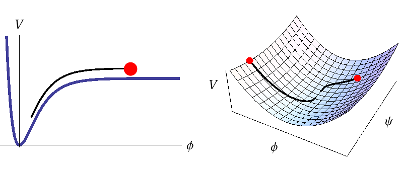
This shows the scalar field potential energy density V as a function of one field (left) or two fields (right). The red dots indicate some possible initial positions for the fields, while the black lines show the paths the fields would take during inflation. With one field you can only go one way down the potential; all initial conditions give the same outcome. With more than one field the paths are different for different initial conditions and each of these predict slightly different statistics for the CMB.
However, fundamental particle physics theories, like string theory or supersymmetry, often have hundreds or thousands of scalar fields. Since these theories become most relevant at energy scales close to the inflationary energy scale, there is considerable interest in analyzing their dynamics. This certainly complicates things. Multifield models have not only one, but usually an infinite number of ways to inflate. The potential energy that drives inflation can now be distributed across any combination of the fields and this distribution of energy changes during the inflationary period in complicated ways that depend on the fields’ initial conditions. The dynamics can even be chaotic! With so many more degrees of freedom, multifield models give a much wider range of possible universes. Understanding whether or not our universe fits into this spectrum is obviously a big challenge!
To determine the predictions of multifield models it is therefore useful to employ a numerical approach that can handle their increased complexity. Over a few visits back-and-forth between London and Auckland, my collaborators and I have built an efficient numerical engine that can solve the exact equations describing the inhomogeneous perturbations. The speed of the code has allowed us to calculate statistics for models with over 200 scalar fields — many more than previously possible. Perhaps surprisingly, our calculations indicate that the most likely predictions of the multifield models are bunched tightly around tiny regions of parameter space and are not sensitively dependent on the initial conditions of the fields.
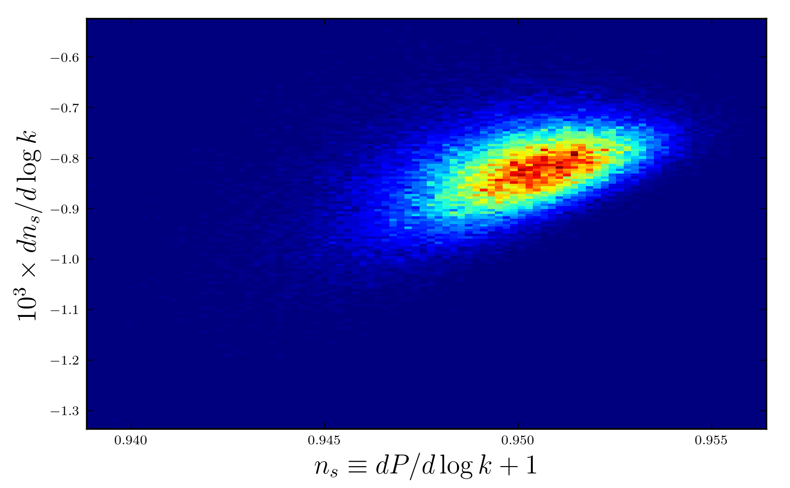
This is a 2D histogram where blue and red indicate less-likely and more-likely regions, respectively. We have used 100 fields to drive inflation and have looked at 100,000 different initial conditions. But first, some basics: simple inflation models predict density perturbations that are random and the density’s modes at a given physical scale, or wavenumber k, are drawn from a Gaussian probability distribution with a variance equal to the primordial power spectrum P(k). A perfect white noise spectrum has P=constant. So, I have plotted here the first and second derivatives of P with respect to the logarithm of k. Although the possibilities for this multifield model are widely varied, the vast majority of our results are grouped tightly together, indicating that the initial conditions are less important than one might expect.
This is important because, in order to calculate how much the observations favor a given model, we need to sample the entire relevant portion of the model’s parameter space and weight each combination of parameters according to how well they fit our CMB observations. This process is computationally difficult, so if we can argue that the fields’ initial conditions only weakly affect the model’s predictions, then it allows us to use a smaller sample, greatly simplifying the calculation.
The end-goal of this line of research is to know which animal in the zoo of inflation models, if any, gives the best description of our universe. For each of these models we must individually calculate the probability that the model is true given the data we have extracted from the CMB — in Bayesian statistics this is known as the posterior probability for the model. By taking the ratio of two models’ posterior probabilities we can determine which model we should bet on being the better description of nature. While we still have more work to do before we can calculate which multifield inflation model is best, we now have many efficient tools in place. There will be much more to come soon!
You can read more here:
R. Easther, J. Frazer, H. V. Peiris, and L. C. Price
Simple predictions from multifield inflationary models
R. Easther and L. C. Price
Initial conditions and sampling for multifield inflation
The scientists working on Planck have been awarded a Physics World Top 10 breakthrough of 2013 “for making the most precise measurement ever of the cosmic microwave background radiation”.
The European Space Agency’s Planck satellite is the first European mission to study the origins of the universe. It surveyed the microwave sky from 2009 to 2013, measuring the cosmic microwave background (CMB), the afterglow of the Big Bang, and the emission from gas and dust in our own Milky Way galaxy. The satellite performed flawlessly, yielding a dramatic improvement in resolution, sensitivity, and frequency coverage over the previous state-of-the-art full sky CMB dataset, from NASA’s Wilkinson Microwave Anisotropy Probe.
The first cosmology data from Planck was released in March 2013, containing results ranging from a definitive picture of the primordial fluctuations present in the CMB temperature, to a new understanding of the constituents of our Galaxy. These results are due to the extensive efforts of hundreds of scientists in the international Planck Collaboration. Here we focus on critical contributions made at UCL to these results.
Planck’s detectors can measure temperature differences of millionths of a degree. To achieve this, some of Planck‘s detectors must be cooled to about one-tenth of a degree above absolute zero – colder than anything in nature – so that their own heat does not swamp the signal from the sky. Giorgio Savini spent the five years prior to launch building the cold lenses as well as testing and selecting all the other optical components which constitute the “eyes” of the Planck High Frequency Instrument. During the first few months of the mission he helped to analyze the data to make sure that the measurements taken in space and the calibration data on the ground were consistent.
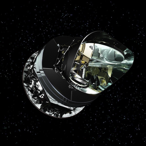
Artist’s rendering of the Planck satellite with view inside the telescope shields. The focal plane unit is visible as the golden collection of waveguide horns at the focus of the telescope positioned inside the thermal shields (external envelope) which protect the telescope from unwanted stray light and aids the cooling of the telescope mirrors by having a black emitting surface on the outside and a reflective one on the inside. For reference, the Earth and Sun would be located far towards the bottom left of this picture. (Credit: ESA/Planck)
UCL researchers Hiranya Peiris, Jason McEwen, Aurélien Benoit-Lévy and Franz Elsner played key roles in using the Planck cosmological data to understand the origin of cosmic structure in the early universe, the global geometry and isotropy of the universe, and the mass distribution of the universe as traced by lensing of the CMB. As a result of Planck’s 50 megapixel map of the CMB, our baby picture of the Universe has sharpened, allowing the measurement of the parameters of the cosmological model to percent precision. As an example, Planck has measured the age of the universe, 13.85 billion years, to half per-cent precision.
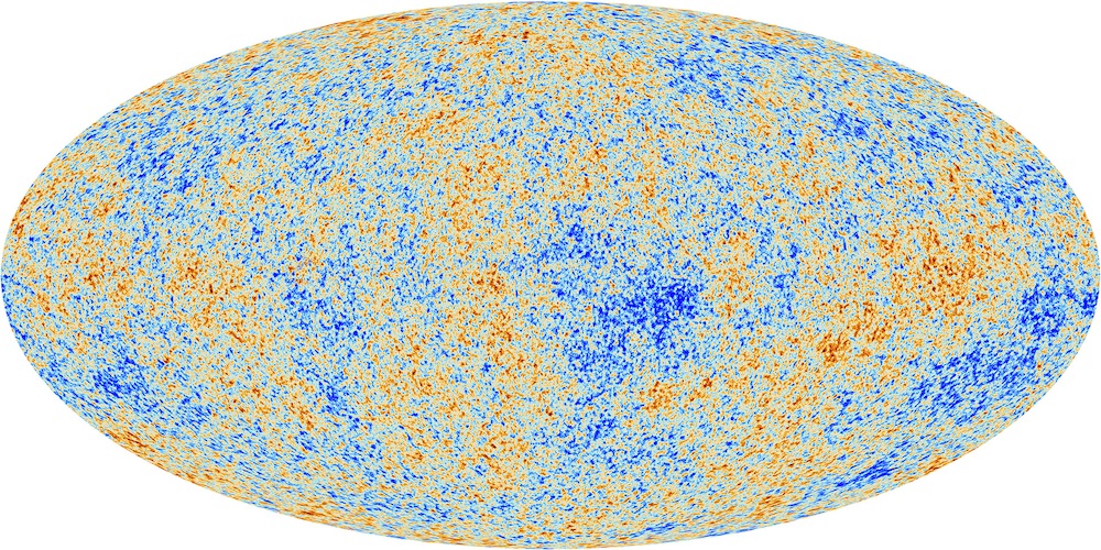
The anisotropies of the cosmic microwave background (CMB) as observed by Planck. The CMB is a snapshot of the oldest light in our Universe, imprinted on the sky when the Universe was just 380 000 years old. It shows tiny temperature fluctuations that correspond to regions of slightly different densities, representing the seeds of all future structure: the stars and galaxies of today. (Credit: ESA/Planck)
The precision of the measurements has also allowed us to rewind the story of the Universe back to just a fraction of a second after the Big Bang. At that time, at energies about a trillion times higher than produced by the Large Hadron Collider at CERN, all the structure in the Universe is thought to have been seeded by the quantum fluctuations of a so-called scalar field, the inflaton. This theory of inflation predicts that the power in the CMB fluctuations should be distributed as a function of wavelength in a certain way. For the first time, Planck has detected, with very high precision, that the Universe has slightly more power on large scales compared with small scales – the cosmic symphony is very slightly bass-heavy, yielding a key clue to the origin of structure in the Universe. Inflation also predicts that the CMB fluctuations will have the statistical properties of a Gaussian distribution. Planck has verified this prediction to one part in 10,000 – this is the most precise measurement we have in cosmology.
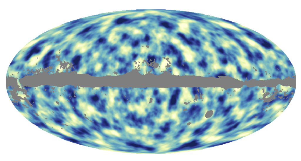
As the CMB photons travel towards us their paths get very slightly bent by massive cosmological structures, like clusters of galaxies, that they have encountered on the way. This effect, where the intervening (dark) matter acts like a lens – only caused by gravity, not glass – on the photons, slightly distorts the CMB. The Planck team was able to analyse these distortions, extract the lensing signature in the data, and create the first full-sky map of the entire matter distribution in our Universe, through 13 billion years of cosmic time. A new window on the cosmos has been opened up.
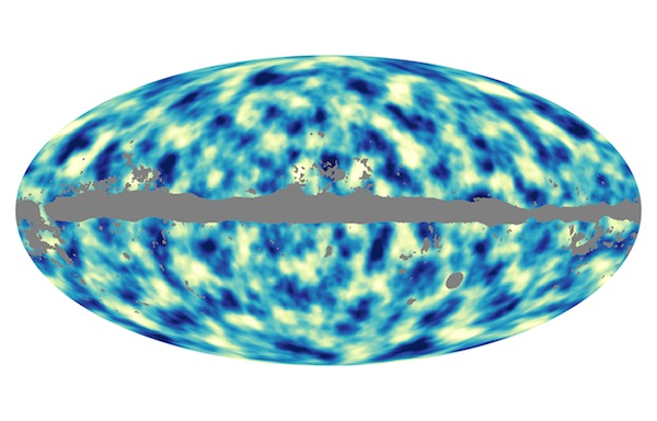
This all-sky image shows the distribution of dark matter across the entire history of the Universe as seen projected on the sky. It is based on data collected with ESA’s Planck satellite during its first 15.5 months of observations. Dark blue areas represent regions that are denser than the surroundings, and bright areas represent less dense regions. The grey portions of the image correspond to patches of the sky where foreground emission, mainly from the Milky Way but also from nearby galaxies, is too bright, preventing cosmologists from fully exploiting the data in those areas. (Credit: ESA/Planck)
Einstein’s theory of general relativity tells us about the local curvature of space-time but it cannot tell us about the global topology of the Universe. It is possible that our Universe might have a non-trivial global topology, wrapping around itself in a complex configuration. It is also possible that our Universe might not be isotropic, i.e., the same in all directions. The exquisite precision of Planck data allowed us to put such fundamental assumptions to the test. The Planck team concluded that our Universe must be close to the standard topology and geometry, placing tight constraints on the size of any non-trivial topology; some intriguing anomalies remain at the largest observable scales, requiring intense analysis in the future.
Aside from additional temperature data not included in the first year results, the upcoming Planck data release in summer 2014 will also include high resolution full-sky polarization maps. This additional information will not only allow us to improve our measurements of the cosmological parameters even further; it will also advance our understanding of our own Galaxy by probing the structure of its magnetic fields and the distribution and composition of dust molecules. There is a further, exciting possibility: if inflation happened, the structure of space should be ringing with primordial gravitational waves, which can be detected in the polarized light of the CMB. We may be able to detect these in the Planck polarization data.
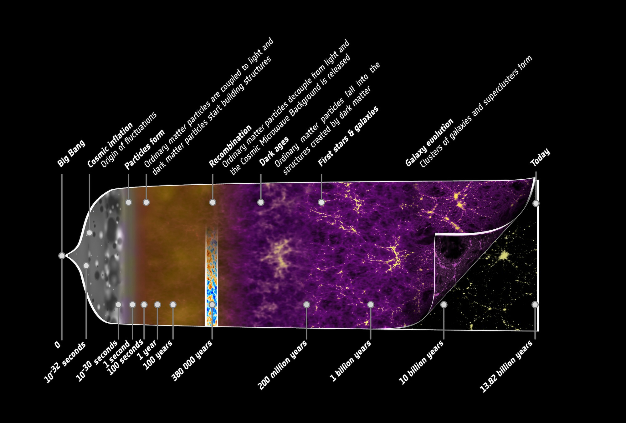
This illustration summarises the almost 14-billion-year long history of our Universe. It shows the main events that occurred between the initial phase of the cosmos, where its properties were almost uniform and punctuated only by tiny fluctuations, to the rich variety of cosmic structure that we observe today, from stars and planets to galaxies and galaxy clusters. (Credit: ESA/Planck)
This guest blog post was written by Max Wainwright.
In modern cosmological models, the very, very early Universe was dominated by a period of exponential growth, known as inflation. As inflation stretched and smoothed the expanding space, particles that were once right next to each other would soon find themselves at the edges of each other’s cosmological horizons, and after that they wouldn’t be able to see each other at all. It was a time of little matter and radiation — an almost complete void except for the immense vacuum energy that drove the expansion.
Luckily, at some point inflation stopped. The vacuum energy decayed into a hot dense plasma soup, which would later cool into particles and, by gravitation, conglomerate into all of the complicated cosmic structure that we see today.
The theory of eternal inflation is quite similar: the very early Universe was dominated by exponential growth, and at some point the growth needed to stop and the energy needed to be converted into matter and radiation. The difference is that in eternal inflation, the growth need not have stopped all at once. Instead, little bubbles of space could have randomly stopped inflating, or fallen onto trajectories which would lead to inflation’s end. The bubbles’ interiors would be in a lower energy state (less vacuum energy means slower inflation), and since they’re in an energetically favorable state they would expand into the inflating exterior. This is much the same as little bubbles of steam growing and expanding in a pot of boiling water: a steam bubble nucleates randomly, and then grows by converting water into more steam. If the Universe weren’t expanding, or if it were expanding slowly, each bubble would eventually run into another bubble and the entire Universe would be converted to the lower vacuum energy. But, in a rapidly expanding universe, the space between bubbles is growing even as the bubbles are themselves growing into that space. If the expansion is fast enough, the growth of inflating space will be faster than its conversion into lower-energy bubbles — inflation will never end.
Signals and Bubble Collisions
Eternal inflation is therefore a theory of many bubble universes individually nucleating and growing inside an ever-expanding background multiverse. If true, eternal inflation would mean that everything that we see, plus a huge amount that we don’t see (hidden behind our cosmological horizon), all came from a single bubble amongst an infinity of other bubbles. Eternal inflation takes the Galilean shift one step further: not only are we not the center of the Universe, but even our universe isn’t the center of the Universe! But how can we ever hope to test this theory?
Most pairs of bubble universes will never collide with each other — they’re too far apart, and the space between them is expanding too fast — but some pairs will form close enough together that they will meet. The ensuing collision will perturb the space-time inside each bubble, and, if we’re lucky, that perturbation may be visible today as a small temperature anisotropy in the cosmic microwave background (CMB).
In a recent paper with my collaborators (M. Johnson, H. Peiris, A. Aguirre, L. Lehner, and S. Liebling) we examined such a possibility. We developed a code that, for the first time, is able to simulate the collision of two bubble universes and follow their evolution all the way to the end of inflation inside each bubble. We then computed the space-time as seen by an observer inside one of the bubbles, and found what the collision would look like on his or her sky.
The model that we use starts with potential energy as a function of a single scalar field. There is a little bump at the top of the potential, forming a local minimum and a barrier. If the field is in the minimum, then it would classically stay there forever. But quantum mechanically the field can tunnel across the barrier — this is the start of a bubble universe. The field inside the bubble will then slowly roll down the potential. The interior will inflate (which is important for matching with standard cosmology), but at a slower rate than the exterior. Once the field reaches the potential’s absolute minimum and the vacuum energy goes to zero, inflation will stop and the kinetic energy in the field will convert into the hot plasma mentioned above (a process known as ‘reheating’).
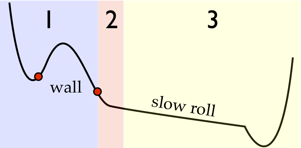
A schematic of the scalar-field potential. Region 1 controls the tunneling behavior. The field, for example, might tunnel from one red dot to another. Region 2 controls the early-time behavior inside each bubble, and therefore also controls the collision behavior between two bubbles. Region 3 controls the slow-roll inflation inside the bubble. Inflation inside the bubble needs to last long enough to solve the horizon and flatness problems in cosmology.
This next figure shows a simulation of a single collision. By symmetry, we only need to simulate one spatial dimension along with the time dimension. The x-axis is the spatial dimension, and the y-axis shows elapsed time (the time-variable N measures the number of e-folds in the eternally inflating vacuum. That is, it measures how many times the vacuum has grown by a factor of e). With our funny choice of coordinates, there is exponentially more space as we go up the graph, so even though it looks like the bubbles asymptote to a fixed size they are physically always getting bigger. You can see that collision can have a drastic effect upon the interior of the bubbles! In this case, the effect is to push the field further down the inflationary potential.
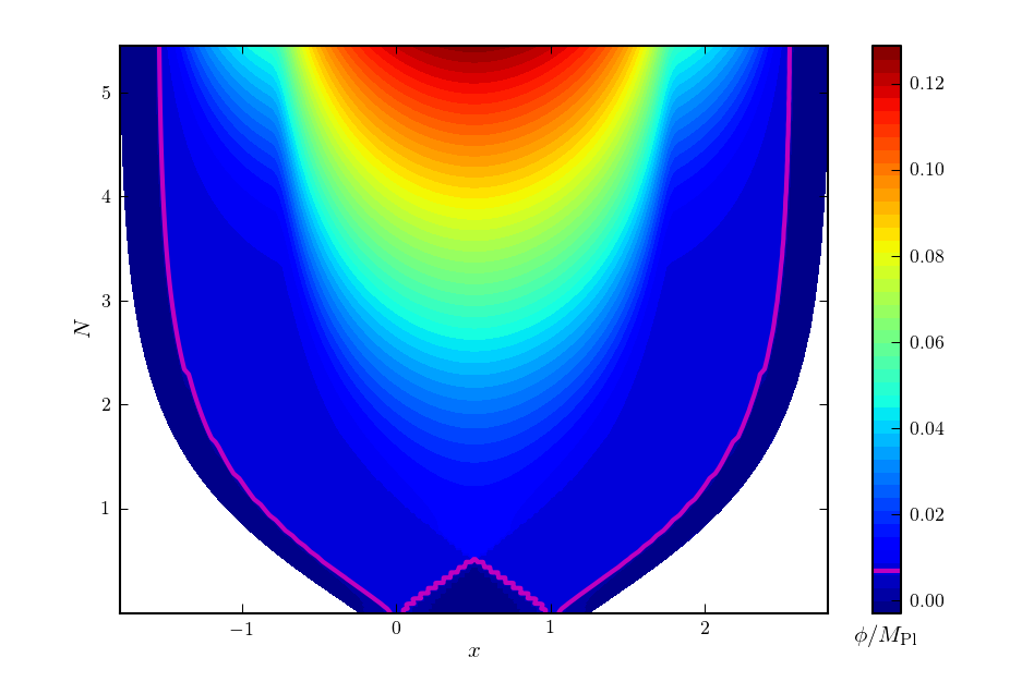
Simulation of colliding bubbles. The pink line shows the bubbles’ exteriors; white space is outside of the simulation. The different colors show different values of the scalar field.
With a collision simulation in hand, we could then figure out what collision actually looks like to an observer residing inside one of the bubbles. This step was pretty complicated — it involved a few tricky coordinate transformations and building up the observer space-time by combining many geodesic trajectories — but the end result was a measure of the comoving curvature perturbation R, which, by the Sachs-Wolfe approximation, is directly proportional to the temperature anisotropy signal that an observer would see in the CMB. The next figure shows a slice of the perturbation across an observer’s coordinates.
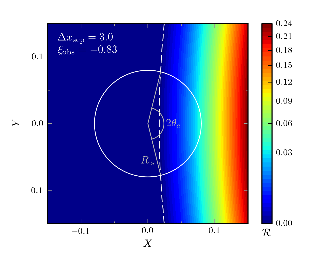
Comoving curvature perturbation near an observer. The perturbation is azimuthally symmetric (symmetric about the X-axis), so the Z-axis does not need to be shown. An observer would see the perturbation on the slice of their past light-cone which intersects the surface of last scattering (the space-time surface from which the CMB is emitted). In the two dimensions plotted here, that surface would (for example) coincide with the circle surrounding the origin. In three dimensions, the collision would look like a big slightly bright spot on one side of the CMB sky.
Predictions and Next Steps
What I’ve shown here is the result of a single bubble collision for a single observer, but, as shown in the paper, we ran many different collisions with different initial separations between bubbles, and found the resulting signal for many different observers. This allowed us to make robust predictions for what sizes and shapes of collisions we should expect to see, given this model. We will then use this information to actually hunt for the collision signals in the sky using data from the Planck space observatory.
So far we’ve only examined one model for how the scalar-field potential should look, but we have no strong theoretical bias to believe that that model is right. Now that we have all of the machinery, we can start examining a slew of different models with different collision properties. Will the collisions generically look the same, or will different models predict very different signals? If we find a signal, what models can it rule out?
It’s an exciting time to be a cosmologist. If we’re lucky, we may soon learn of our proper place in the multiverse.
You can read more here:
C. L. Wainwright, M. C. Johnson, H. V. Peiris, A. Aguirre, L. Lehner, S. L. Liebling
Simulating the universe(s): from cosmic bubble collisions to cosmological observables with numerical relativity
M. C. Johnson, H. V. Peiris, L. Lehner
Determining the outcome of cosmic bubble collisions in full General Relativity
S. M. Feeney, M. C. Johnson, J. D. McEwen, D. J. Mortlock, H. V. Peiris
Hierarchical Bayesian Detection Algorithm for Early-Universe Relics in the Cosmic Microwave Background
This blog post was written by Andrew Pontzen and originally published by astrobites. Hiranya Peiris will be writing a response exploring why she believes that both rapid and slow expansion are confusing, and giving her take on explaining the inflationary picture to non-specialists – watch this space!
Loading the post. If this message doesn’t disappear, please check that javascript is enabled in your browser.
Cosmic inflation is a hypothetical period in the very early universe designed to solve some weaknesses in the big bang theory. But what actually happens during inflation? According to wikipedia and other respectable sources, the main effect is an ‘extremely rapid’ expansion. That stock description is a bit puzzling; in fact, the more I’ve tried to understand it, the more it seems like inflation is secretly all about slow expansion, not rapid expansion. The secret’s not well-kept: once you know where to look, you can find a note by John Peacock that supports the slow-expansion view, for example. But with the rapid-expansion picture so widely accepted and repeated, it’s fun to explore why slow-expansion seems a better description. Before the end of this post, I’ll try to recruit you to the cause by means of some crafty interactive javascript plots.
A tale of two universes
There are many measurements which constrain the history of the universe. If, for example, we combine information about how fast the universe is expanding today (from supernovae, for example) with the known density of radiation and matter (largely from the cosmic microwave background), we pretty much pin down how the universe has expanded. An excellent cross-check comes from the abundance of light elements, which were manufactured in the first few minutes of the universe’s existence. All-in-all, it’s safe to say that we know how fast the universe was expanding all the way back to when it was a few seconds old. What happened before that?
Assuming that the early universe contained particles moving near the speed of light (because it was so hot), we can extrapolate backwards. As we go back further in time, the extrapolation must eventually break down when energies reach the Planck scale. But there’s a huge gap between the highest energies at which physics has been tested in the laboratory and the Planck energy (a factor of a million billion or so higher). Something interesting could happen in between. Inflation is the idea that, because of that gap, there may have been a period during which the universe didn’t contain particles. Energy would instead be stored in a scalar field (a similar idea to an electric or magnetic field, only without a sense of direction). The Universe scales exponentially with time during such a phase; the expansion rate accelerates. (Resist any temptation to equate ‘exponential’ or ‘accelerating’ with ‘fast’ until you’ve seen the graphs.) Ultimately the inflationary field decays back to particles and the classical picture resumes. By definition, all is back to normal long before the universe gets around to mundane things like manufacturing elements. For our current purposes, it’s not important to see whether inflation is a healthy thing for a young universe to do (wikipedia lists some reasons if you’re interested). We just want to compare two hypothetical universes, both as simple as possible:
- a universe containing fast-moving particles (like our own once did);
- as (1), but including a period of inflation.
Comparisons are odorous
There are a number of variables that might enter the comparison:
- a: the scalefactor, i.e. the relative size of a given patch of the universe at some specified moment;
- t: the time;
- da/dt: the rate at which the scalefactor changes with time;
- or if you prefer, H: the Hubble rate of expansion, which is defined as d ln a / dt.
We’ll take a=1 and t=0 as end conditions for the calculation. There’s no need to specify units since we’re only interested in comparative trends, not particular values. There are two minor complications. First, what do we mean by ‘including inflation’ in universe (2)? To keep things simple it’ll be fine just to assume that the pressure in the universe instantaneously changes. (Click for a slightly more specific description.) The change will kick in between two specified values of a — that is, over some range of ‘sizes’ of the universe. In particular, taking the equation of state of the universe to be pressure = w × density × c2, we will assume w=1/3 except during inflation, when w= –1. The value of w will switch instantaneously at a=a0, and switch back at a=a1. (Click for details of the transition.)The density just carries over from the radiation to the inflationary field and back again (as it must, because of energy-momentum conservation). In reality, these transitions are messy (reheating at the end of inflation is an entire topic in itself) – but that doesn’t change the overall picture.
Finding the plot
The Friedmann equations (or equivalently, the Einstein equations) take our history of the contents of the universe and turn it into a history of the expansion (including the exponential behaviour during inflation). But now the second complication arises: such equations can only tell you how the Hubble expansion rate H (or, equivalently, da/dt) changes over time, not what its actual value is. So to compare universes (1) and (2), we need one more piece of information – the expansion rate at some particular moment. Since we never specified any units, we might as well take H=1 in universe (1) at t=0 (the end of our calculation). Any other choice is only different by a constant scaling. What about universe (2)? As discussed above, the universe ends up expanding at a known rate, so really universe (2) had better end up expanding at the same rate as universe (1). But, for completeness, you’ll be able to modify that choice below and have universe (1) and (2) match their expansion rate at any time. All that’s left is to choose the variables to plot. I’ve provided a few options in the applet below. It seems they all lead to the conclusion that inflation isn’t ultra-rapid expansion; it’s ultra-slow expansion. By the way, if you’re convinced by the plots, you might wonder why anyone ever thought to call inflation rapid. One possible answer is that the expansion back then was faster than at any subsequent time. But the comparison shows that this is a feature of the early universe, not a defining characteristic of inflation. Have a play with the plots and sliders below and let me know if there’s a better way to look at it.
This plot shows the Hubble expansion rate as a function of the size of the universe. A universe with inflation (solid line) has a Hubble expansion rate that is slower than a universe without (dashed line). Inflation is a period of slow expansion! In the current plot, sometimes the inflationary universe (solid line) is expanding slower, and sometimes faster than the universe without inflation (dashed line). But then, you’ve chosen to make the Hubble rate exactly match at an arbitrary point during inflation, so that’s not so surprising. Currently it looks like the inflationary universe (solid line) is always expanding faster than the non-inflationary universe (dashed line). But the inflationary universe ends up (at a=1) expanding much faster than H=1, which was our target based on what we know about the universe today. So there must be something wrong with this comparison.
This plot shows the size of the universe as a function of time. Inflationary universes (solid line) hit a=0 at earlier times. In other words, a universe with inflation (solid line) is always older than one without (dashed line) and has therefore expanded slower on average. Inflation is a period of slow expansion! With the current setup you’re not matching the late-time expansion history in the inflationary universe against the known one from our universe; to make a meaningful comparison, the dotted and solid lines must match at late times (t=0). So the plot can’t be used to assess the speed of expansion during inflation.
This plot shows the Hubble expansion rate of the universe. The universe with an accelerating period (solid line) is always expanding at the same rate or slower than the one without (dashed line). Inflation is a period of slow expansion! Currently it looks like the inflationary universe (solid line) may expand faster than the non-inflationary universe (dashed line). But the inflationary universe ends up (at t=0) expanding much faster than H=1, which was our target based on what we know about the universe today. So there must be something wrong with this comparison.
This plot shows the rate of change of scalefactor (da/dt) as a function of time before the present day. The universe with an accelerating period (solid line) is always expanding at the same rate or slower than the one without (dashed line). Inflation is a period of slow expansion! With the current setup you’re not matching the late-time expansion history in the inflationary universe (solid line) against the known one from our universe (da/dt does not match at t=0, for instance). So the plot can’t be used to assess the speed of expansion during inflation.
First select the range of scalefactors over which inflation occurs by dragging the two ends of the grey bar. Currently, a0=X and a1=X
In realistic models of inflation, this range would extend over many orders of magnitude in scale, making the effects bigger than the graphs suggest.
Now select the scalefactor at which the expansion rate is matched between universe (1) and (2).
At the moment amatch=X: you’re matching after inflation is complete. That makes sense because various observations fix the expansion rate at this time.
At the moment amatch=X: you’re matching before or during inflation. Look at the Hubble rate at the end of inflation and you’ll find it disagrees between the two universes. That means they can’t both match what we know about the universe at late times, so the comparison isn’t really going to be fair.
Acknowledgements
Pedro Ferreira, Tom Whyntie, Nina Roth, Daniela Saadeh, Steven Gratton, Nathan Sanders, Rob Simpson, and Jo Dunkley made helpful comments on an early version. Rob Simpson and Brooke Simmons pointed me to the javascript libraries d3, rickshaw and numeric.
As usual, this time of year is a very busy one for EarlyUniverse @ UCL, with several departures and new arrivals! We bid a fond farewell to Dr Stephen Feeney, who moves to Imperial College London to work with Andrew Jaffe. Stephen’s thesis, titled “Novel Algorithms for Early Universe Cosmology”, won the Jon Darius Memorial Prize at UCL recently.
Stephen Feeney and Hiranya Peiris at Stephen’s PhD graduation.
We also say goodbye to Dr Jonny Frazer, who spent a short but highly productive time as a postdoc at UCL. Several exciting papers are in the pipeline from his time at UCL, and we will be blogging about this work in coming months. Jonny moves to the theory group at Bilbao, Spain, where he will be honing his kite-surfing skills inbetween doing physics!
Jason McEwen’s leaving do and new faculty position celebration.
Dr Jason McEwen has just moved as a Lecturer to our sister department, the Mullard Space Science Laboratory at UCL. Fortunately, he will still be blogging for us! We also welcome Dr Andrew Pontzen, a brand-new Lecturer at UCL Physics and Astronomy. Last but not least, we are very excited to have three new postdocs on board: Drs Franz Elsner, Marc Manera, and Nina Roth, as well as new PhD student Daniela Saadeh. We are looking forward to their upcoming blog posts!
Halloween carvings.
Keeping up our tradition at this time of year, a few members of EarlyUniverse @ UCL got together for a Halloween pumpkin-carving party. Here is their handiwork!
Hiranya Peiris has been named one of 10 “Rising Stars of Astronomy” by Astronomy Magazine in their July 2013 issue! Read more here.
This blog post was written by Aurélien Benoit-Lévy.
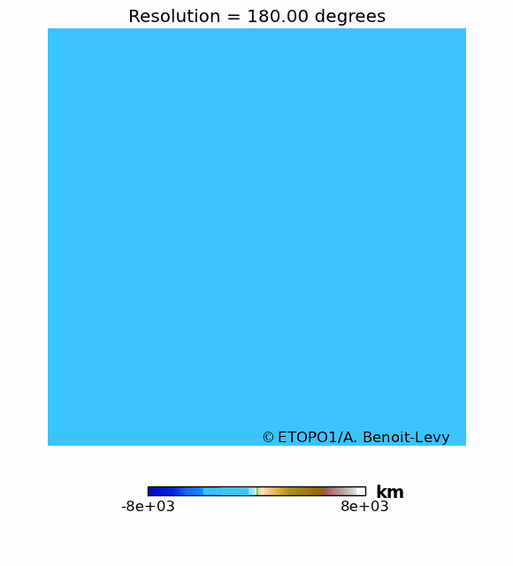
There’s a lot of activity on this blog about the cosmic microwave background (CMB) and Planck, and on how much Planck has improved our view of the baby universe compared to its predecessors WMAP and COBE. One of the things that have drastically improved between those satellites is the angular resolution. This simply means that Planck is able to see finer details in the CMB and is therefore able to extract more cosmological information.
However, getting the physical sense of a finite resolution instrument is not always easy, especially since we don’t know what the CMB fluctuations should look like. That’s why we can use a familiar object and play around with the resolution parameter. So let’s consider our planet Earth, which indeed we know quite well!
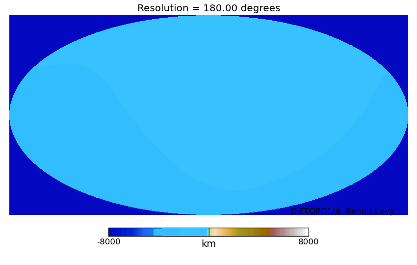
So, what would the Earth look like if it was seen by a satellite with an angular resolution similar to that of COBE (about 7 degrees), WMAP (about 14 arc-minutes), or Planck (5 arc-minutes)? Let’s first clarify what we mean by observation of the Earth by a satellite. We can very easily find online topographic data of the Earth that indicates the altitude of continents and the depth of seabeds. Let’s now make the following analogy: instead of having a satellite that measures the energy (or temperature) of the photons of the CMB, we have a satellite that measures the altitude of the Earth, this altitude being negative when we’re looking at oceans. And then, we can create a map of the altitude of the Earth:
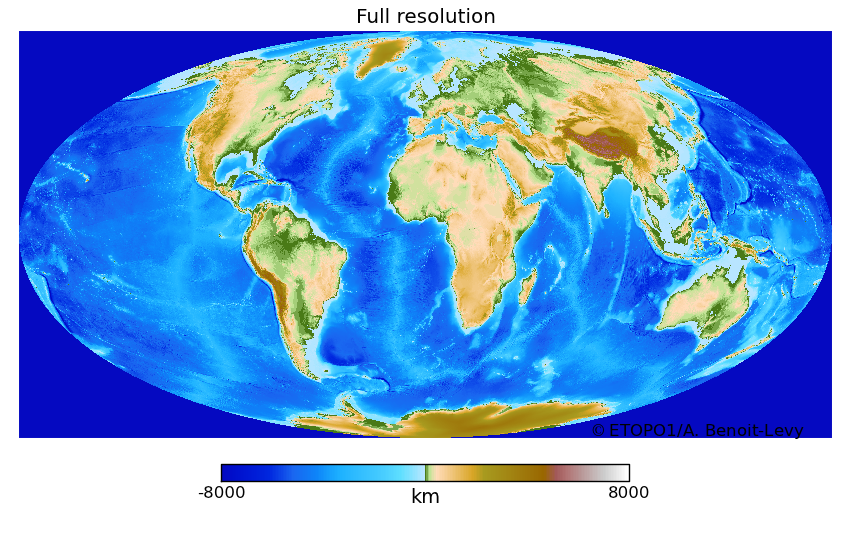
Full resolution map, given by the resolution of the initial data of about 1 arc-minute.
The following animation shows the Earth as seen first by a very basic satellite that would only be sensitive to structure at the scale of 180 degrees. At this scale, the only thing we can see is the average altitude of the Earth, and that is why the animation starts with a monotonic blue map. The resolution can therefore be thought of as the scale at which details are smoothed and cannot be easily discerned. Then the resolution increases (i.e., the smallest visible altitude decreases, I know that’s confusing), and we see the highest regions of the Earth coming into view one by one: first the Himalayas, and then the Antarctic, and all the other mountains.
At the COBE resolution (7 degrees) we can distinguish the large continents, but we cannot resolve finer details like the South-East Asian Islands or Japan. Another interesting fact is that it seems that there’s not much difference between the Planck and WMAP resolutions. That is mostly because the image is too small to be sensitive to such fine resolution, and thus we need to zoom in, in order to see the improvement of Planck compared to WMAP.
We can now concentrate on an even more familiar region. The following figures show how the British Isles would appear as seen by COBE, WMAP, Planck, and the original data.
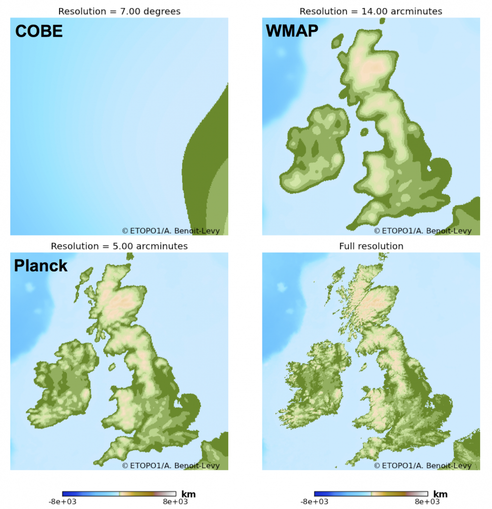
And this comes quite as a surprise: at the COBE resolution, England is totally overpowered by France, and does not seem to exist at all! This might actually be a good thing if harmful aliens were to observe the Earth at COBE resolution before launching an attack: they would not spot England and would strike at France!
More seriously, we have seen previously that, at the 7 degree resolution, islands are not yet resolved and are hidden by the high mountains that spread their intensity (in this case their altitude) over large angular distances. However, at WMAP resolution the British Isles are perfectly resolved but everything appears blurred. The situation improves with Planck resolution and then we can see the improvement between WMAP and Planck. Note that even at the Planck resolution, we miss fine details and there is much more information in the original data. That is, however, not the case for the CMB, as physical processes at recombination actually damp the signal at small scales, and Planck indeed extracts all the information in the primary CMB.
To conclude this post, the following animation shows the “Rise of the British Isles”.
The topographic data is from the ETOPO1 global relief website, and could in principle be found here.
Hiranya Peiris talking about what it’s like being a cosmologist, the recent results from the Planck satellite and the interplay between cosmology and the Higgs boson discovery at CERN, as part of a series of interviews for Origins 2013, a European Researcher’s Night event.
This blog post was written by Jason McEwen.
The standard model of cosmology assumes that the Universe is homogenous (i.e. the same everywhere) and isotropic (i.e. the same in whichever direction we look). However, are such fundamental assumptions valid? With high-precision cosmological observations, we can put these fundamental assumptions to the test.
Recently we have studied models of rotating universes, the so-called Bianchi models, in order to test the isotropy of the Universe. In these scenarios, a subdominant contribution is embedded in the temperature fluctuations of the cosmic microwave background (CMB), the relic radiation of the Big Bang. We therefore search for a weak Bianchi component in WMAP and Planck observations of the CMB – we know any Bianchi component in the CMB must be small since otherwise we would have noticed it already!
Intriguingly, a weak Bianchi contribution was found previously in WMAP data. Even more remarkably, this component seemed to explain some of the so-called ‘anomalies’ reported in WMAP data. We since developed a rigorous Bayesian statistical analysis technique to quantify the overall statistical evidence for Bianchi models from the latest WMAP data and the recent Planck data.
When we consider the full physical model, where the standard and Bianchi cosmologies are coherent and fitted to the data simultaneously, we find no evidence in support of Bianchi models from either WMAP or Planck – the enhanced complexity of Bianchi models over the standard cosmology is not warranted. However, when the Bianchi component is treated in a phenomenological manner and is decoupled from the standard cosmology, we find a Bianchi component in both WMAP and Planck data that is very similar to that found previously (see plot).
So, is the Universe rotating? Well, probably not. It is only in the unphysical scenario that we find evidence for a Bianchi component. In the physical scenario we find no need to include Bianchi models.
However, only very simple Bianchi models have been compared to the data so far. There are more sophisticated Bianchi models that more accurately describe the physics involved and could perhaps even provide a better explanation of CMB observations.
We’re looking into it!
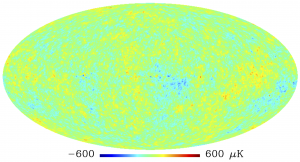
WMAP full-sky CMB data
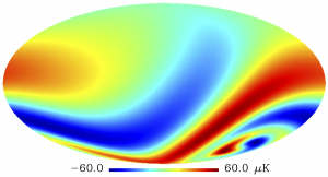
Unphysical Bianchi component embedded in the CMB
You can read more here:
J. D. McEwen, T. Josset, S. M. Feeney, H. V. Peiris, A. N. Lasenby
Bayesian analysis of anisotropic cosmologies: Bianchi VII_h and WMAP
T. R. Jaffe, A. J. Banday, H. K. Eriksen, K. M. Gorski, F. K. Hansen
Evidence of vorticity and shear at large angular scales in the WMAP data: a violation of cosmological isotropy?
Planck Collaboration
Planck 2013 results. XXVI. Background geometry and topology of the Universe
A. Pontzen, A. Challinor
Bianchi Model CMB Polarization and its Implications for CMB Anomalies
This blog post was written by Jonathan Frazer.
The pigeon problem
In 1964, Bell Labs built a new antenna which was designed to detect the radio waves bounced from echo balloon satellites, but there was a problem with the antenna. The signal was far less clean than they were expecting. The first theory seeking to explain this signal was the pigeon droppings theory. A pair of pigeons had built a nest in the antenna and so the hypothesis was that by removing these pigeons, the signal would be improved.
In general, one of the perks of being a cosmologist is that there are very few ethical issues to worry about. I am sad to say however that in this instance, extreme measures were taken. The pigeons were shot. What is more, they died in vain since the noisy signal persisted. The pigeon droppings theory was ruled out.
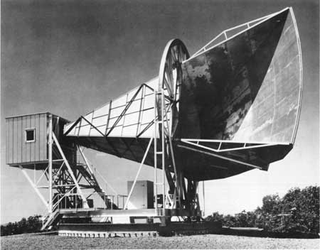
The Holmdel Horn Antenna. Photo Credit: Bell Labs
At this point a new theory became popular. Rather than the unwanted signal being caused by pigeon waste, it was now proposed that the source of contamination could be explained by a controversial theory known as the Big Bang. Largely the result of philosophical bias, for a long time it had been thought that the Universe had always existed, staying much the same for all eternity. This new theory proposed there was in some sense a beginning to our Universe. A particularly nice feature of this theory was that it had a number of striking predictions relating to the fact that soon after the Universe came into existence, it would be very hot and very dense. One of these predictions was that a simple series of cosmic events would take place as the universe expanded, and this would result in radiation that should be observable even today. It was this radiation that caused the problem at Bell Labs.
The problem of predictability
This radiation, often referred to as the cosmic microwave background (CMB) is remarkable in many ways and plays a role of paramount importance in testing both theories of the early universe, and theories of late time structure formation. One important characteristic is that almost nothing has interfered with this radiation since its creation; it is essentially a snapshot of the universe, soon after its birth.
This brings me to the problems we face today, and hence also the work I have done in my thesis. There is a beautiful theory of the early universe known as inflation. This theory describes how quantum fluctuations are the seeds that eventually grow to become the complex structures we see today, such as galaxies, stars and even life. In order to test this theory, it is essential that we understand with great precision how these quantum fluctuations will be imprinted in the CMB. A significant part of my work to date has been to develop better methods of doing this.
However, testing the theory of inflation has turned out to be rather more challenging than first expected. As I mentioned, the early universe was very hot and very dense which means that any theory of the early universe inevitably involves studying particle physics at energy scales far far greater than anything we could ever hope reproduce in an experiment on Earth. This means we must study particle physics at a more fundamental level. This leads us to string theory!
String theory famously suffers from the problem that it is exceedingly difficult to test experimentally. So the prospect that there may be information encoded in the CMB, for many physicists, is very exciting! That said, there is a serious problem. Historically, theories of inflation were very simple and much like the pigeon theory, they were easy to test. Typically there would be only one species of particle that needed to be considered and this would mean it was straightforward to make a prediction. However, again much like the pigeon theory, it seems these theories are too basic and the reality may be significantly more complex. Recent developments in string theory have resulted in inflationary models becoming vastly more complex. Often containing tens if not hundreds of fields which need to be taken into account, this has resulted in a class of models where it is no longer understood how to make predictions.
Fortunately there is reason to think this challenge can be overcome. While the underlying structure of this new class of models can be exceedingly complicated, the combined effect of all the messy interactions between these many particles can actually result in a wonderfully simple and consistent behaviour. It is far too soon to say whether or not this result is generic but this emergent simplicity may hold the key to understanding how string theory can finally be tested!
Jonathan Frazer
Predictions in multifield models of inflation, submitted to JCAP.
Mafalda Dias, Jonathan Frazer, Andrew R. Liddle
Multifield consequences for D-brane inflation, JCAP06(2012)020.
David Seery, David J. Mulryne, Jonathan Frazer, Raquel H. Ribeiro
Inflationary perturbation theory is geometrical optics in phase space, JCAP09(2012)010.
Jonathan Frazer and Andrew R. Liddle
Multi-field inflation with random potentials: field dimension, feature scale and non-Gaussianity, JCAP02(2012)039.
Jonathan Frazer and Andrew R. Liddle
Exploring a string-like landscape, JCAP02(2011)026.
The cosmology conference LSS13 on “Theoretical Challenges for the Next Generation of Large-Scale Structure Surveys” took place in the beautiful city of Ascona in Switzerland between June 30 and July 5. It brought together experts in the theory, simulation and data analysis of galaxy surveys for studying the large-scale structure of the universe.
Boris attended LSS13 and presented his work on cosmology with quasar surveys. Thanks to good preparation (and a lot of feedback from colleagues at UCL), Boris won the award for the best contribution/presentation from a young researcher! This award not only included a framed certificate, but also a T shirt and a small cash prize! The picture below captures this moment with the organisers of the conference, Professors Uros Seljak and Vincent Desjaques, in front of the sculpture that symbolises the Centro Stefano Franscini in Ascona.
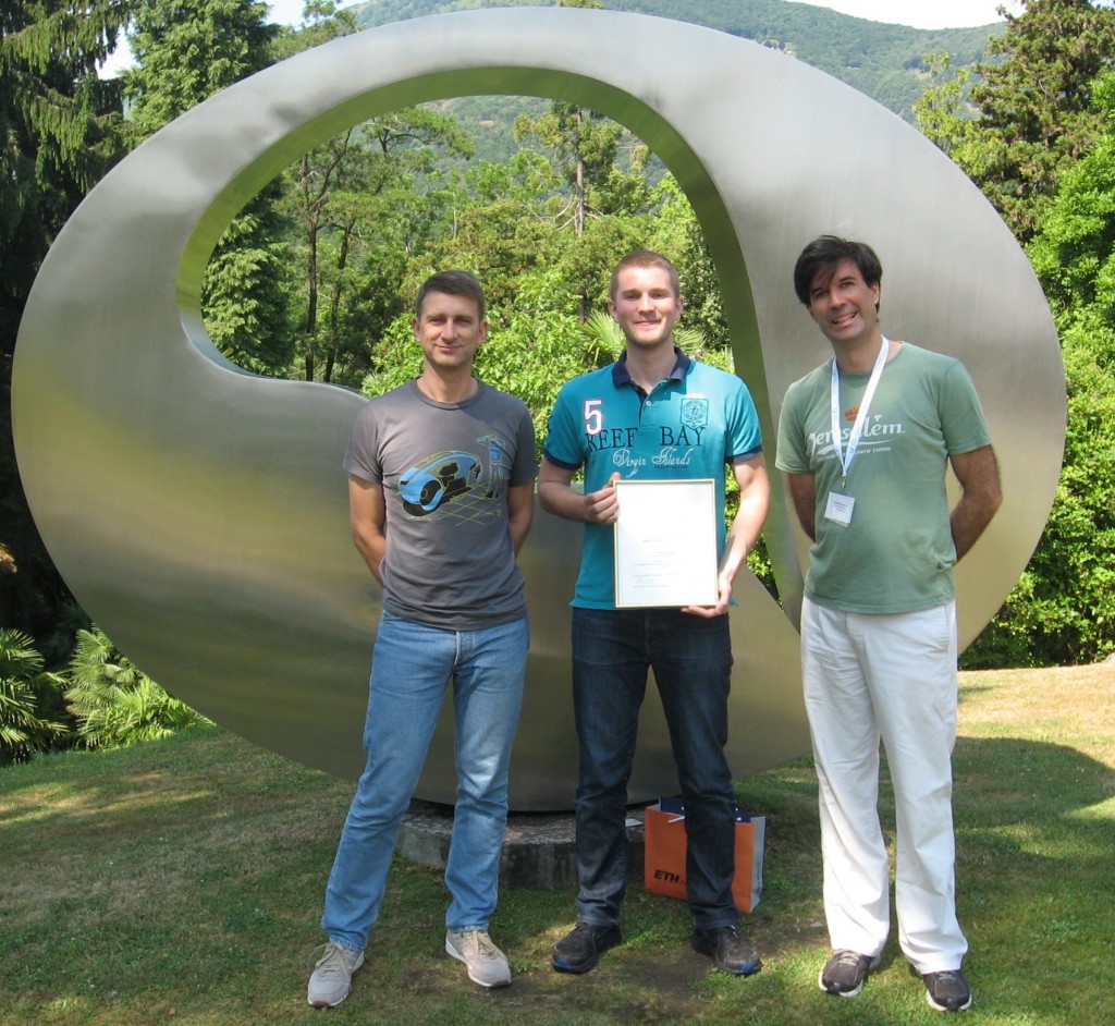
Boris and the conference organisers, Professors Uros Seljak (left) and Vincent Desjaques (right), posing in front of the conference center in Ascona.
This blog post was written by Boris Leistedt.
Devoured from within by supermassive black holes, quasars are among the most energetic and brightest objects in the universe. Their light sometimes travels several billion years before reaching us, and by looking at how they cluster in space, cosmologists are able to test models of the large-scale structure of the universe. However, being compact and distant objects, quasars look like stars and can only be definitively identified using high-resolution spectroscopic instruments. However, due to the time and expense of taking spectra, not all star-like objects can be examined with these instruments, and quasar candidates first need to be identified in a photometric survey and then confirmed or dismissed by taking follow-up spectra. This approach has led to the identification and study of tens of thousands of quasars, greatly enhancing our knowledge of the physics of these extreme objects.
Current catalogues of confirmed quasars are too small to study the large-scale structure of the universe at sufficient precision. For this reason, cosmologists use photometric catalogues of quasar candidates in which each object is only characterised by a small set of photometric colours. Star-quasar classification is difficult, yielding catalogues that in fact contain significant fractions of stars. In addition, the unavoidable variations in the calibration of instruments and in the observing conditions over time, create fluctuations in the number and properties of star-like objects detected on the sky. These observational issues combined with stellar contamination result in distortions in the data that can be misinterpreted as anomalies or hints of new physics.
In recent work we investigated these issues, and demonstrated techniques to address them. We considered the photometric quasars from the Sloan Digital Sky Survey (SDSS) and selected a subsample of objects where 95% of objects were expected to be actual quasars. We then constructed sky masks to remove the areas of the sky which were the most affected by calibration errors, fluctuations in the observing conditions, and dust in our own Galaxy. We exploited a technique called “mode projection” to obtain robust measurements of the clustering of quasars, and compared them with theoretical predictions. Using this, we found a remarkable agreement between the data and the prediction from the standard model of cosmology. Previous studies of such data argued that they were not suitable for cosmological studies, but we were able to identify a sample of objects that appear clean. In the future, we will use these techniques to analyse future photometric data, for example in the context of the Dark Energy Survey in which UCL is deeply involved.
Photometric quasars and some of their systematics
Hiranya Peiris recently gave a talk at TEDxCERN, CERN’s first event under the TEDx program.
You can watch her talk, titled The Universe: a Detective Story, here. Enjoy!
Continuing EarlyUniverse@UCL’s tradition of recognition by the Royal Astronomical Society, Stephen Feeney has been named runner-up for the Michael Penston Prize 2012, awarded for the best doctoral thesis in astronomy and astrophysics. Stephen’s PhD thesis (“Novel Algorithms for Early Universe Cosmology”) focused on constraining the physics of the very early Universe — processes such as eternal inflation and the formation of topological defects — using novel Bayesian source-detection techniques applied to cosmic microwave background data. Stephen is extremely happy and completely gobsmacked to have been recognised!

This blog post was written by Aurélien Benoit-Lévy.
In my previous post, I mentioned CMB lensing and said that it was going to be a big thing. And indeed, CMB lensing has been presented as one of the main scientific results of the recent data release from the Planck Collaboration. So what is CMB lensing? Put succinctly, CMB lensing is the deflection of CMB photons as they pass clumps of matter on the way from the last scattering surface to our telescopes. These deflections generate a characteristic signature in the CMB that can be used to map out the distribution of all of the matter in our Universe in the direction of each incoming photon. Let me now describe these last few sentences in greater detail.
I am sure you are familiar with images of distorted and multiply-imaged galaxies observed around massive galaxy clusters. All of these images are due to the bending of light paths by changes in the distribution of matter, an effect generally known as gravitational lensing. The same thing happens with the CMB: the trajectories of photons coming from the last scattering surface are modified by gradients in the distribution of matter along the way: i.e. the large-scale structure of our Universe.
The main effect is that the CMB we observe is sightly modified: the temperature we measure in a certain direction is actually the temperature we would have measured in a slightly different direction if there were no matter in the Universe. These deflections are small — about two arcminutes, or the size of a pixel in the full-resolution Planck map — and can hardly be distinguished by eye. Indeed, if you look at the nice animation by Stephen Feeney, it not possible to say which is the lensed map and which is the unlensed map. But there’s one thing we can see, and that’s that the deflections are not random. If you concentrate on one big spot (either blue or red) you’ll see that it moves coherently in one single direction. The coherence of these arcminute deflections over a few degrees is extremely important as it enables us to estimate a quantity known as the lensing potential: the sum of all the individual deflections experienced by a photon as it travels from the last scattering surface. Although we can only measure the net deflection, rather than the full list of every deflection felt by the photon, the lensing potential still represents the deepest measurement we can have of the matter distribution as it probes the whole history of structure formation!
Now, how can we extract this lensing potential from a CMB temperature map? As I mentioned earlier, CMB lensing generates small deflections (a few arcminutes) but correlated on larger scales (a few degrees). This mixing of scales (small and large) results from small non-Gaussianities induced by CMB lensing. More precisely, the CMB temperature and its gradient become correlated, and this correlation is given precisely by the lensing potential. We can therefore measure the correlation between the temperature and the gradient of a CMB map to provide an estimate of the lensing potential. Of course, this operation is not straightforward and there are quite a lot of complications due to the fact that the data are not perfect. But we can model all of these effects, and, as they are largely independent of CMB lensing, they can be easily estimated using simulations and then simply removed from the final results.
It’s as simple as that! However, there’s much more still to come as I haven’t yet spoken of the various uses of this lensing potential! But that’s another story for another time…
The Planck lensing potential. This map can be thought as a the map of the matter in our Universe projected on the sky.
This blog post was written by Hiranya Peiris.
There was great excitement at EarlyUniverse@UCL this week due to the first cosmology data release from the Planck satellite! Andrew Jaffe has a nice technical guide to the results here, and Phil Plait has a great, very accessible summary here.
The data and papers are publicly available, and you can explore Planck’s stunning maps of the fossil heat of the Big Bang – the cosmic microwave background (CMB) – on the wonderful Chromoscope.
Planck’s results bring us much closer to understanding the origin of structure in the universe, and its subsequent evolution. In the past few months, Jason McEwen, Aurélien Benoit-Lévy and I have been working extremely hard on the Planck analyses studying the implications of the data for a range of cosmological physics. Now we can finally talk publicly about this work, and in coming weeks we will be blogging about these topics; but in the meantime the technical papers are linked below!
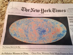
The Planck results received wide media coverage, including the BBC, The Guardian, the Financial Times, the Economist, etc. But as a former part-time New Yorker, the most thrilling moment of the media circus for me was seeing Planck’s CMB map taking up most of the space above the fold, on the front page of the New York Times!
You can read more here:
Planck Collaboration (2013):
Planck 2013 results. XVI. Cosmological parameters
Planck 2013 results. XVII. Gravitational lensing by large-scale structure
Planck 2013 results. XXII. Constraints on inflation
Planck 2013 results. XXIII. Isotropy and Statistics of the CMB
Planck 2013 Results. XXIV. Constraints on primordial non-Gaussianity
Planck 2013 results. XXV. Searches for cosmic strings and other topological defects
Planck 2013 results. XXVI. Background geometry and topology of the Universe
This guest blog post was written by Aurélien Benoit-Lévy.
The cosmic microwave background (CMB) is the furthest light we can observe. Since it is the furthest, bright galaxies and other compact objects can pollute in a nasty way the superb observations of the CMB that forthcoming experiments will soon deliver. To get rid of these point sources, we need to mask them. This is of course not harmless, as the resulting map is punched with holes just like emmental!
Holes in a map are unfortunate as they considerably complicate the spectral properties of the signal under consideration. But if there is a problem somewhere, it means that there is a solution, and I’m sure you would have guessed the solution: inpainting! Inpainting is just like cod, it’s good when it’s well made. The basic idea is to fill the holes with some fake data that would mimic some properties of the original signal. There are plenty of methods to inpaint a hole. For instance, the simplest one would be to fill the hole with the mean of all the surrounding pixels, but we can do much better than that.
CMB has a nice property: it’s correlated. This means that the probability that a given pixel has a given value is not independent of the value of the other pixels. And the CMB is also (very very close to) Gaussian, so we can use those two properties to generate random constrained Gaussian realizations that mimic the lost signal, but preserve the statistical structure of the map. Basically, we can use the information contained in the non-contaminated region to guess the most probable value in the holes. This technique has been known for quite a while, but sometimes requires heavy computations to accurately take into account all the information available in the map.
In recent work, my collaborators and I have demonstrated that it is not necessary to account for the whole map to inpaint a small hole. Using only the neighboring pixels is enough. With this method, we are able to inpaint a realistic CMB map, with a realistic point source mask in a realistic time! And the statistical properties of the inpainted maps are virtually unchanged! We applied this locally-constrained Gaussian realization in the special case of CMB lensing reconstruction and showed that this tool is very efficient, as it preserves the two-point statistic, and – above all – does not generate a spurious four-point signal. Of course, I now need to tell you about CMB lensing and four-point statistics, which is a very big thing and we’ll hear a lot about it in the coming months. But that will be for another post!
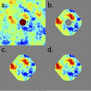
(a) CMB map with a point source hole, (b) neighbouring pixels used to inpaint the hole, (c) Input map, (d) Inpainted map
You can read more here:
Aurélien Benoit-Lévy et al.
Full-sky CMB lensing reconstruction in the presence of sky-cuts.
This guest blog post was written by Stephen Feeney.
Neutrinos are puzzling little particles. The Standard Model of particle physics tells us that there are three different types, or “flavours”, of neutrinos, each of which has no mass. Particle physics experiments, however, tell a different story. Firstly, the fact that neutrinos produced in the Sun (and nuclear reactors) are observed to oscillate between flavours requires them to have mass. Furthermore, unexpected results corroborated by a number of experiments measuring the rate of oscillations hint at the existence of more than three neutrino flavours.
This is all very interesting, and it seems that the Standard Model is ripe for revision, but what has it got to do with cosmology? Quite a lot, as it happens! Neutrinos, along with all fundamental particles, are produced in the early Universe. As they are so light, the neutrinos are extremely relativistic, and hence very energetic: so much so that, along with the photons, they dominate the dynamics of the early Universe. If there are four neutrinos rather than the standard three, the Universe initially expands more quickly than the current cosmological model (LambdaCDM) predicts, and cold dark matter becomes important at later times. Furthermore, neutrinos are so energetic that they are able to escape from the density perturbations set up in the early Universe — they “free-stream” a certain distance which is dependent on their mass — and hence affect the amount of structure that forms.
All of this has observable consequences for cosmology, affecting the relative amounts of simple elements produced in the Universe’s first few minutes, the amplitude and scale of the oscillations in the cosmic microwave background (CMB), and the numbers of, for example, galaxy clusters. We can therefore try to determine the number of neutrino species and their masses from cosmology! In fact, the strength of the effects of neutrinos in the early Universe, coupled with the quality of cosmological data, means that cosmological tests of neutrino physics are more powerful than laboratory experiments.
That’s what we (Hiranya, Licia Verde and I) have been doing. People have, of course, already started looking for hints of non-standard neutrinos in cosmology, and have found weak indications that the most likely number of neutrino species is greater than three. These analyses have, however, relied on parameter estimates: finding the most likely number of neutrino species given the data, and claiming evidence of new physics if this is not the standard value.
What we really want to do is to determine the support for a model with, for example, extra neutrinos, and compare this to the support for the standard cosmological model. This is what we’ve done: we have used the Bayesian evidence to compare the relative probabilities of LambdaCDM and models with extra neutrino flavours and massive neutrinos, given cosmological data. The datasets we consider include CMB power spectra from WMAP and the South Pole Telescope, measurements of the Universe’s recent expansion, and measurements of the weak gravitational lensing of the CMB by intervening large-scale structure. Our model-selection results indicate that the standard cosmological model is favoured over models with additional neutrinos and/or neutrino mass. There is therefore no requirement from cosmology to change our view of the neutrino. We’re going to need better cosmological data — such as the Planck data coming in a couple of months’ time — to make progress on this problem.
The lensing of the CMB by intervening matter: a promising cosmological probe of neutrino properties.
You can read more here:
Stephen M. Feeney, Hiranya V. Peiris and Licia Verde
Is there evidence for additional neutrino species from cosmology? JCAP, submitted, 2013.
Paul Sutter is visiting UCL this week to collaborate on the detection and cosmological uses of cosmic voids using wavelet methods. He kindly wrote a guest blog for EarlyUniverse@UCL.
Voids are all the large, empty spaces in the Universe. Until recently they have been mostly ignored as astronomers focused on all the bright, hot, and glowy stuff out there: stars, galaxies, and clusters. And we can’t really blame the astronomers: stars, galaxies, and clusters are easy to spot, easy to collect information from, have rich dynamics…in other words, they’re interesting.
Voids, on the other hand, are hard to identify, hard to collect information from, and have relatively uninteresting dynamics. In fact, they are so boring that their structure and evolution pretty much echoes the early universe with very little modification. This yields a surprising result: if we can reliably identify voids, then we have an almost perfectly clear window into the early universe and the nature of dark energy!
Galaxy surveys such as the Sloan Digital Sky Survey are mapping large volumes of the Universe, revealing many structures large and small, including cosmic voids. Working with Ben Wandelt and Guilhem Lavaux, I’ve adapted a void finder to work with real observational data.
The figure shows the distribution of medium-sized voids in our nearby universe. In the figure, the points are individual galaxies. With the additional help of David Weinberg, I’ve developed a public catalog of these voids. This catalog is accelerating many kinds of innovative void-based science.
More information can be found at cosmicvoids.net and pmsutter.com.
Voids in the SDSS. Copyright Paul Sutter.
Written by visiting collaborator and guest blogger Matt Johnson.
Computer simulations of the early universe allow us to explore scenarios that are just not possible to examine using pencil-and-paper calculations. I was recently in London working on how to use computer simulations to predict the observable signatures of eternal inflation. In the standard story of eternal inflation, our universe is purported to be enclosed inside one bubble among many, each expanding into an inflating background space-time. Our bubble undergoes collisions with others, providing a possible observational window on this bizarre scenario (read about the latest tests in this paper).
The field configuration making up our bubble determines the properties of our cosmology. For example, the symmetry of a single bubble fixes the universe to be an open Friedmann-Robertson-Walker (FRW) space-time. However, the collision between bubbles upsets this symmetry, meaning that if we live inside a bubble which underwent collisions, there will be deviations from a purely open FRW space-time.
The equations governing the evolution of the fields making up the bubbles and gravity are highly non-linear, making computer simulations a necessary tool for finding the exact space-time resulting from the collision between bubbles. Setting our sights on understanding the collision between pairs of bubbles, there is enough symmetry to evolve in 1 space and 1 time dimension. Last year, we wrote a code to simulate the collision between two bubble universes (you can read about our first results in this paper). One shortcoming of this original work was that the coordinates we used prevented us from evolving for longer than a few e-folds of inflation. We’ve fixed that by introducing a more appropriate set of coordinates, and now the challenge is to extract the cosmology contained inside one of the bubbles.
For colliding bubbles, one no longer has a purely homogeneous and isotropic cosmology. However, if collisions are to be consistent with what we observe, there had better be regions where the space-time is approximately FRW. So, how does one identify which regions are approximately FRW from the simulation data? How does one then quantify the deviation from FRW, so that quantitative predictions can be made? Our current method tracks the behaviour of geodesics evolved through the simulation. Because we know how geodesics would evolve through a purely FRW universe, we can determine the qualitative and quantitative differences. This is depicted schematically in the figure below, where I’ve shown the results of a simulation, and some of the geodesics evolving in the background. The geodesics entering the affected region pile up, indicating a deviation from pure FRW. We hope to polish the final code off soon, and extract the first observational signatures from our simulations!

The anatomy of a bubble collision
Jason McEwen recently gave a talk at CALIM 2012 (CALibration and IMaging for the SKA) on the application of compressive sensing techniques to imaging for radio interferometry.
You can watch his talk here. Enjoy!
Stephen Feeney passed his PhD viva on Nov 15th! His thesis is entitled “Novel Algorithms for Early Universe Cosmology”. Congratulations to Dr Feeney!
The newly minted Dr Feeney, with the supporting cast (left to right) of Boris Leistedt, Filipe Abdalla, Jason McEwen, and Hiranya Peiris.
It has been a very busy autumn for Early Universe @UCL, but we took time out to celebrate Halloween with a pumpkin carving competition! Jason, the esteemed judge, says:
So, the results from the pumpkin carving competition are now in…
We have two categories: best geek homage and best teeth. Entries were received from Hiranya and Boris.

“Ghostly Moon Landing”, by Hiranya Peiris
Hiranya’s entry: “Ghostly moon landing” in honour of Neil Armstrong.

“Miam Miam”, by Boris Leistedt
Boris’ entry: “Miam miam”, which according to Boris translates as “yum yum”.
In the best geek homage category, Boris’ entry comes a respectable 3rd and the grand prize goes to… Hiranya!
In the best teeth category, Hiranya’s entry comes a respectable 3rd and the grand prize goes to… Boris!
Surprisingly, it’s almost as if the participants tailored their entries to each category! In any case, it turns out everyone’s a winner! Yay!
Last May, Boris Leistedt and Jason McEwen finished developing the first exact harmonic and wavelet transforms in 3D spherical coordinates. The paper has now been peer-reviewed and will be published in IEEE Trans. Sig. Proc. in December. The code is available on www.flaglets.org.
Why exact? Exact transforms are essential in information sciences because they enable one to capture all the information contained in a complex signal, and process it without any loss of information. Thanks to this theoretical property, the accuracy achieved by the transform is only limited by the representation of floating-point numbers on the computer!
Why wavelets? Wavelet transforms are increasingly successful in various disciplines (including astrophysics and geophysics) because they separate scale-dependent, localised features in the signals of interest, which is very suited to the extraction of patterns in complex data. As an example they were used by Stephen Feeney and Hiranya Peiris to search for potential signatures of topological defects in the cosmic microwave background.
Why in three dimensions? In astrophysics, spherical wavelets are naturally suited to the analysis of signals on the sky, and cosmologists have already started to apply them to galaxy surveys, for instance to help dealing with the systematics or to isolate structures at different physical scales of interest. However galaxy surveys are 3D datasets where the angular position is accurately measured on the sky but the radial information (such as photometric redshift or distance) is often estimated from color information and therefore subject to uncertainty. Not only one should use 3D wavelets to properly treat such data, but these wavelets should furthermore separate the radial and angular features to avoid mixing of radial and tangential systematic uncertainties. The accuracy would also be critical because most modern pipelines apply these transforms repeatedly (to go back and forth from pixel to wavelet space), leading to a loss of information if the transform is not exact.
3D sampling theorem for the Fourier-Laguerre transform
What is the outcome? To address these problems, Boris and Jason designed a 3D harmonic transform combined with a sampling theorem on the ball, namely a 3D pixelization scheme that captures all the harmonic information in a finite set of samples on the ball. Then, they defined wavelet kernels, called “flaglets”, to extract scale-dependent, localised features in signals defined on the ball. The flaglets isolate patterns in the radial and angular dimensions separately and are very promising for analysing galaxy surveys and treating their systematics.
The code is fast, accurate, and is publicly available on www.flaglets.org.

Flaglet transform of a N-body simulation. The top left signal is the input data, and the following signals are the flaglets. Click on the image to see larger version.
Cosmic bubble collisions provide an important observational window on the dynamics of eternal inflation. In eternal inflation, our observable universe is contained in one of many bubbles formed from an inflating metastable vacuum. The collision between bubbles can leave a detectable imprint on the cosmic microwave background (CMB) radiation. Although phenomenological models of the observational signature have been proposed, to make the theory fully predictive one must determine the bubble collision spacetime, and thus the cosmological observables, from a scalar field theory giving rise to eternal inflation. Numerical simulations of bubble collisions in full General Relativity (GR) are needed to make a direct connection between a scalar field model giving rise to eternal inflation and the signature of bubble collisions expected to be present in the CMB. Numerics are important because the collision between bubbles is a highly non-linear process.
We recently took the first steps towards this goal, in collaboration with Matt Johnson and Luis Lehner at the Perimeter Institute in Canada. We simulated collisions between two bubbles in full GR. These simulations allowed us to accurately determine the outcome of bubble collisions, and examine their effect on the cosmology inside a bubble universe. Studying both vacuum bubbles and bubbles containing a realistic inflationary cosmology, we confirmed the validity of a number of approximations used in previous analytic work, and identified qualitatively new features of bubble collision spacetimes, such as oscillons. We identified the constraints on the scalar field potential that must be satisfied in order to obtain collisions that are consistent with our observed cosmology, yet leave detectable signatures.
The figures below show a couple of examples of bubble collisions in our simulations.
An example of a collision between two vacuum bubbles. The bubble on the left, which has lower energy than the one on the right, “wins” in the collision, eating into the other bubble. Oscillons form at the interface between the two bubbles.
An example of a collision between bubbles containing an inflationary cosmology. The colour-coding of the contours shows that the scalar field receives a “kick” to the future of the collision.
![]()


Axisymmetric wavelets on the sphere
Wavelets are a powerful signal analysis tool due to their ability to localise signal content in scale and position simultaneously. The generic nature of wavelets means that they are suitable for many problems, but by the same token, for certain problems they are not necessarily optimal. In some instances, where we have a good prior knowledge of the signal we are interested in, we can create an optimal filter to look for it.
When looking for the signatures of bubble collisions in cosmic microwave background (CMB) observations, we have a good theoretical prediction of the expected form of the signal. To detect likely bubble collisions candidates in the CMB, we developed a source detection algorithm using optimal filters.
Since the bubble collision signatures that we expect to see in the CMB vary with size and position on the sky, wavelets are a powerful method for the candidate source detection, and indeed have been shown to work very well.


Optimal matched filters on the sphere
The image below shows the signal-to-noise ratio (SNR) achieved by wavelets and optimal filters for detecting bubble collisions in the CMB. We see that optimal filters outperform wavelets since they are closely adapted to the profile of both the bubble collision signature and also the background stochastic process (the CMB).
For the detection of cosmic bubble collisions, optimal filters allow us to exploit our knowledge of the expected signal. However, wavelets are suitable for a wider class of problems. As always, the best analysis technique to adopt depends heavily on the problem at hand.
Signal-to-noise ratio achieved for detecting bubble collision signatures in the CMB using wavelets (black dot-dashed) and optimal filters (blue solid), compared to looking at the original data (red dashed)
